[latex]x[/latex]-intercepts of a Function and Solutions of an Equation

How can we find the [latex]x[/latex]-intercepts (or real zeros) of a function [latex]y=f(x)[/latex]? First, we need to set [latex]y=0[/latex] because all [latex]x[/latex]-intercepts are on the [latex]x[/latex]-axis and any points on the [latex]x[/latex]-axis have zero for its [latex]y[/latex]-coordinate. Then, we need to solve the equation [latex]f(x)=0[/latex]. For example, to find the [latex]x[/latex]-intercepts (or real zeros) of a function [latex]f(x)=\frac{1}{7}x(x+3)(x-5)[/latex], we need to solve the equation [latex]\frac{1}{7}x(x+3)(x-5)=0[/latex]. From this equation, we can find [latex]x=-3, 0, 5[/latex] as its solutions and can write them as [latex](-3, 0)[/latex], [latex](0, 0)[/latex], and [latex](5, 0)[/latex] because those solutions are the [latex]x[/latex] values when its [latex]y[/latex] value is zero. So, we can conclude that the solutions of the equation [latex]\frac{1}{7}x(x+3)(x-5)=0[/latex] is actually the [latex]x[/latex]-intercepts (or real zeros) of the function [latex]f(x)=\frac{1}{7}x(x+3)(x-5)[/latex]. We can confirm this relation from the graph of the function [latex]f(x)=\frac{1}{7}x(x+3)(x-5)[/latex] as well.

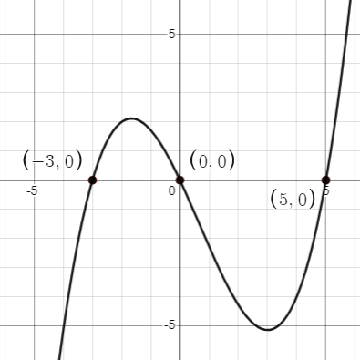
Figure 2. Graph of [latex]f(x)=\frac{1}{7}x(x+3)(x-5)[/latex]

In Figure 2, we can find the solutions of the equation [latex]\frac{1}{7}x(x+3)(x-5)=0[/latex] by locating the [latex]x[/latex]-intercepts of the graph of the function [latex]f(x)=\frac{1}{7}x(x+3)(x-5)[/latex].

Distinct Parts of a Graph of a Function

Now let’s consider more points on the graph. As we can see in Figure 2, some parts of the graph are above the [latex]x[/latex]-axis, some parts of the graph are on the [latex]x[/latex]-axis, and some parts of the graph are below the [latex]x[/latex]-axis. Try the following DESMOS activity to explore the relationship between those distinct parts of the function and the sign of its [latex]y[/latex] values:

From the DESMOS activity above, we can conclude the followings: