A monetary policy that lowers interest rates and stimulates borrowing is known as an expansionary monetary policy or easy (loose) monetary policy. Conversely, a monetary policy that raises interest rates and reduces borrowing in the economy is a contractionary monetary policy or tight monetary policy. This module will discuss how expansionary and contractionary monetary policies affect interest rates and aggregate demand, and how such policies will affect macroeconomic goals like unemployment and inflation. We will conclude with a look at the Fed’s monetary policy practice in recent decades.
 |
Learning Objectives
|
The Effect of Monetary Policy on Interest Rates
Consider the market for loanable bank funds, shown in Fig. 1. The original equilibrium (E0) occurs at an interest rate of 8% and a quantity of funds loaned and borrowed of $10 billion. An expansionary monetary policy will shift the supply of loanable funds to the right from the original supply curve (S0) to S1, leading to an equilibrium (E1) with a lower interest rate of 6% and a quantity of funds loaned of $14 billion. Conversely, a contractionary monetary policy will shift the supply of loanable funds to the left from the original supply curve (S0) to S2, leading to an equilibrium (E2) with a higher interest rate of 10% and a quantity of funds loaned of $8 billion.

So how does a central bank “raise” interest rates? When describing the monetary policy actions taken by a central bank, it is common to hear that the central bank “raised interest rates” or “lowered interest rates.” We need to be clear about this: more precisely, through open market operations the central bank changes bank reserves in a way which affects the supply curve of loanable funds. As a result, interest rates change, as shown in Fig.1. If they do not meet the Fed’s target, the Fed can supply more or less reserves until interest rates do.
Recall that the specific interest rate the Fed targets is the federal funds rate. The Federal Reserve has, since 1995, established its target federal funds rate in advance of any open market operations.
Of course, financial markets display a wide range of interest rates, representing borrowers with different risk premiums and loans that are to be repaid over different periods of time. In general, when the federal funds rate drops substantially, other interest rates drop, too, and when the federal funds rate rises, other interest rates rise. However, a fall or rise of one percentage point in the federal funds rate—which remember is for borrowing overnight—will typically have an effect of less than one percentage point on a 30-year loan to purchase a house or a three-year loan to purchase a car. Monetary policy can push the entire spectrum of interest rates higher or lower, but the specific interest rates are set by the forces of supply and demand in those specific markets for lending and borrowing.
The Effect of Monetary Policy on Aggregate Demand
Monetary policy affects interest rates and the available quantity of loanable funds, which in turn affects several components of aggregate demand. Tight or contractionary monetary policy that leads to higher interest rates and a reduced quantity of loanable funds will reduce two components of aggregate demand. Business investment will decline because it is less attractive for firms to borrow money, and even firms that have money will notice that, with higher interest rates, it is relatively more attractive to put those funds in a financial investment than to make an investment in physical capital. In addition, higher interest rates will discourage consumer borrowing for big-ticket items like houses and cars. Conversely, loose or expansionary monetary policy that leads to lower interest rates and a higher quantity of loanable funds will tend to increase business investment and consumer borrowing for big-ticket items.
If the economy is suffering a recession and high unemployment, with output below potential GDP, expansionary monetary policy can help the economy return to potential GDP. Fig.2 (a) illustrates this situation. This example uses a short-run upward-sloping Keynesian aggregate supply curve (SRAS). The original equilibrium during a recession of E0 occurs at an output level of 600. An expansionary monetary policy will reduce interest rates and stimulate investment and consumption spending, causing the original aggregate demand curve (AD0) to shift right to AD1, so that the new equilibrium (E1) occurs at the potential GDP level of 700.

Conversely, if an economy is producing at a quantity of output above its potential GDP, a contractionary monetary policy can reduce the inflationary pressures for a rising price level. In Fig.2 (b), the original equilibrium (E0) occurs at an output of 750, which is above potential GDP. A contractionary monetary policy will raise interest rates, discourage borrowing for investment and consumption spending, and cause the original demand curve (AD0) to shift left to AD1, so that the new equilibrium (E1) occurs at the potential GDP level of 700.
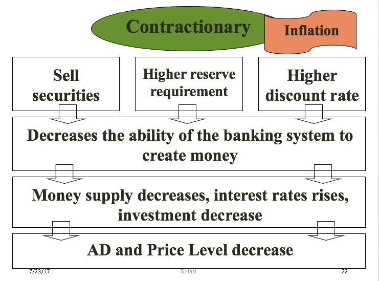
These examples suggest that monetary policy should be countercyclical; that is, it should act to counterbalance the business cycles of economic downturns and upswings. Monetary policy should be loosened when a recession has caused unemployment to increase and tightened when inflation threatens. Of course, countercyclical policy does pose a danger of overreaction. If loose monetary policy seeking to end a recession goes too far, it may push aggregate demand so far to the right that it triggers inflation. If tight monetary policy seeking to reduce inflation goes too far, it may push aggregate demand so far to the left that a recession begins. Fig. (a) summarizes the chain of effects that connect loose and tight monetary policy to changes in output and the price level.

 |
 |
Quantitative Easing
The most powerful and commonly used of the three traditional tools of monetary policy—open market operations—works by expanding or contracting the money supply in a way that influences the interest rate. In late 2008, as the U.S. economy struggled with recession, the Federal Reserve had already reduced the interest rate to near-zero. With the recession still ongoing, the Fed decided to adopt an innovative and nontraditional policy known as quantitative easing (QE). This is the purchase of long-term government and private mortgage-backed securities by central banks to make credit available so as to stimulate aggregate demand.
Quantitative easing differed from traditional monetary policy in several key ways. First, it involved the Fed purchasing long term Treasury bonds, rather than short term Treasury bills. In 2008, however, it was impossible to stimulate the economy any further by lowering short term rates because they were already as low as they could get. Therefore, Bernanke sought to lower long-term rates utilizing quantitative easing.
This leads to a second way QE is different from traditional monetary policy. Instead of purchasing Treasury securities, the Fed also began purchasing private mortgage-backed securities, something it had never done before. During the financial crisis, which precipitated the recession, mortgage-backed securities were termed “toxic assets,” because when the housing market collapsed, no one knew what these securities were worth, which put the financial institutions which were holding those securities on very shaky ground. By offering to purchase mortgage-backed securities, the Fed was both pushing long term interest rates down and also removing possibly “toxic assets” from the balance sheets of private financial firms, which would strengthen the financial system.
Quantitative easing (QE) occurred in three episodes:
Shortcomings of Monetary Policy
In the real world, effective monetary policy faces a number of significant hurdles. Monetary policy affects the economy only after a time lag that is typically long and of variable length. Remember, monetary policy involves a chain of events: the central bank must perceive a situation in the economy, hold a meeting, and make a decision to react by tightening or loosening monetary policy. The change in monetary policy must percolate through the banking system, changing the quantity of loans and affecting interest rates. When interest rates change, businesses must change their investment levels and consumers must change their borrowing patterns when purchasing homes or cars. Then it takes time for these changes to filter through the rest of the economy.
As a result of this chain of events, monetary policy has little effect in the immediate future; instead, its primary effects are felt perhaps one to three years in the future. The reality of long and variable time lags does not mean that a central bank should refuse to make decisions. It does mean that central banks should be humble about taking action, because of the risk that their actions can create as much or more economic instability as they resolve.
Excess Reserves – Cyclical Asymetry
Banks are legally required to hold a minimum level of reserves, but no rule prohibits them from holding additional excess reserves above the legally mandated limit. For example, during a recession banks may be hesitant to lend, because they fear that when the economy is contracting, a high proportion of loan applicants become less likely to repay their loans.
When many banks are choosing to hold excess reserves, expansionary monetary policy may not work well. This may occur because the banks are concerned about a deteriorating economy, while the central bank is trying to expand the money supply. If the banks prefer to hold excess reserves above the legally required level, the central bank cannot force individual banks to make loans. Similarly, sensible businesses and consumers may be reluctant to borrow substantial amounts of money in a recession, because they recognize that firms’ sales and employees’ jobs are more insecure in a recession, and they do not want to face the need to make interest payments. The result is that during an especially deep recession, an expansionary monetary policy may have little effect on either the price level or the real GDP.
Japan experienced this situation in the 1990s and early 2000s. Japan’s economy entered a period of very slow growth, dipping in and out of recession, in the early 1990s. By February 1999, the Bank of Japan had lowered the equivalent of its federal funds rate to 0%. It kept it there most of the time through 2003. Moreover, in the two years from March 2001 to March 2003, the Bank of Japan also expanded the money supply of the country by about 50%—an enormous increase. Even this highly expansionary monetary policy, however, had no substantial effect on stimulating aggregate demand. Japan’s economy continued to experience extremely slow growth into the mid-2000s.
Unpredictable Movements of Velocity
Velocity is a term that economists use to describe how quickly money circulates through the economy. The velocity of money in a year is defined as:
Specific measurements of velocity depend on the definition of the money supply being used. Consider the velocity of M1, the total amount of currency in circulation and checking account balances. In 2009, for example, M1 was $1.7 trillion and nominal GDP was $14.3 trillion, so the velocity of M1 was 8.4 ($14.3 trillion/$1.7 trillion). A higher velocity of money means that the average dollar circulates more times in a year; a lower velocity means that the average dollar circulates fewer times in a year.
Deflation occurs when the rate of inflation is negative; that is, instead of money having less purchasing power over time, as occurs with inflation, money is worth more. Deflation can make it very difficult for monetary policy to address a recession.
Remember that the real interest rate is the nominal interest rate minus the rate of inflation. If the nominal interest rate is 7% and the rate of inflation is 3%, then the borrower is effectively paying a 4% real interest rate. If the nominal interest rate is 7% and there is deflation of 2%, then the real interest rate is actually 9%. In this way, an unexpected deflation raises the real interest payments for borrowers. It can lead to a situation where an unexpectedly high number of loans are not repaid, and banks find that their net worth is decreasing or negative. When banks are suffering losses, they become less able and eager to make new loans. Aggregate demand declines, which can lead to recession.
In the U.S. economy during the early 1930s, deflation was 6.7% per year from 1930–1933, which caused many borrowers to default on their loans and many banks to end up bankrupt, which in turn contributed substantially to the Great Depression. Not all episodes of deflation, however, end in economic depression. Japan, for example, experienced deflation of slightly less than 1% per year from 1999–2002, which hurt the Japanese economy, but it still grew by about 0.9% per year over this period. Indeed, there is at least one historical example of deflation coexisting with rapid growth. The U.S. economy experienced deflation of about 1.1% per year over the quarter-century from 1876–1900, but real GDP also expanded at a rapid clip of 4% per year over this time, despite some occasional severe recessions.
Then the double-whammy: After causing a recession, deflation can make it difficult for monetary policy to work. Say that the central bank uses expansionary monetary policy to reduce the nominal interest rate all the way to zero—but the economy has 5% deflation. As a result, the real interest rate is 5%, and because a central bank cannot make the nominal interest rate negative, expansionary policy cannot reduce the real interest rate further. In the U.S. economy during the early 1930s, deflation was 6.7% per year from 1930–1933, which caused many borrowers to default on their loans and many banks to end up bankrupt, which in turn contributed substantially to the Great Depression. Not all episodes of deflation, however, end in economic depression.
Japan, for example, experienced deflation of slightly less than 1% per year from 1999–2002, which hurt the Japanese economy, but it still grew by about 0.9% per year over this period. Indeed, there is at least one historical example of deflation coexisting with rapid growth. The U.S. economy experienced deflation of about 1.1% per year over the quarter-century from 1876–1900, but real GDP also expanded at a rapid clip of 4% per year over this time, despite some occasional severe recessions.
The central bank should be on guard against deflation and, if necessary, use expansionary monetary policy to prevent any long-lasting or extreme deflation from occurring. Except in severe cases like the Great Depression, deflation does not guarantee economic disaster.
Changes in velocity can cause problems for monetary policy. To understand why, rewrite the definition of velocity so that the money supply is on the left-hand side of the equation. That is:
Recall that
Therefore,
This equation is sometimes called the basic quantity equation of money but, as you can see, it is just the definition of velocity written in a different form. This equation must hold true, by definition.
If velocity is constant over time, then a certain percentage rise in the money supply on the left-hand side of the basic quantity equation of money will inevitably lead to the same percentage rise in nominal GDP—although this change could happen through an increase in inflation, or an increase in real GDP, or some combination of the two. If velocity is changing over time but in a constant and predictable way, then changes in the money supply will continue to have a predictable effect on nominal GDP. If velocity changes unpredictably over time, however, then the effect of changes in the money supply on nominal GDP becomes unpredictable.
The actual velocity of money in the U.S. economy as measured by using M1, the most common definition of the money supply, is illustrated in Fig. 1. From 1960 up to about 1980, velocity appears fairly predictable; that is, it is increasing at a fairly constant rate. In the early 1980s, however, velocity as calculated with M1 becomes more variable. The reasons for these sharp changes in velocity remain a puzzle. Economists suspect that the changes in velocity are related to innovations in banking and finance which have changed how money is used in making economic transactions: for example, the growth of electronic payments; a rise in personal borrowing and credit card usage; and accounts that make it easier for people to hold money in savings accounts, where it is counted as M2, right up to the moment that they want to write a check on the money and transfer it to M1. So far at least, it has proven difficult to draw clear links between these kinds of factors and the specific up-and-down fluctuations in M1. Given many changes in banking and the prevalence of electronic banking, M2 is now favored as a measure of money rather than the narrower M1.

In the 1970s, when velocity as measured by M1 seemed predictable, a number of economists, led by Nobel laureate Milton Friedman(1912–2006), argued that the best monetary policy was for the central bank to increase the money supply at a constant growth rate. These economists argued that with the long and variable lags of monetary policy, and the political pressures on central bankers, central bank monetary policies were as likely to have undesirable as to have desirable effects. Thus, these economists believed that the monetary policy should seek steady growth in the money supply of 3% per year. They argued that a steady rate of monetary growth would be correct over longer time periods, since it would roughly match the growth of the real economy. In addition, they argued that giving the central bank less discretion to conduct monetary policy would prevent an overly activist central bank from becoming a source of economic instability and uncertainty. In this spirit, Friedman wrote in 1967: “The first and most important lesson that history teaches about what monetary policy can do—and it is a lesson of the most profound importance—is that monetary policy can prevent money itself from being a major source of economic disturbance.”
As the velocity of M1 began to fluctuate in the 1980s, having the money supply grow at a predetermined and unchanging rate seemed less desirable, because as the quantity theory of money shows, the combination of constant growth in the money supply and fluctuating velocity would cause nominal GDP to rise and fall in unpredictable ways. The jumpiness of velocity in the 1980s caused many central banks to focus less on the rate at which the quantity of money in the economy was increasing, and instead to set monetary policy by reacting to whether the economy was experiencing or in danger of higher inflation or unemployment.
Unemployment and Inflation
If you were to survey central bankers around the world and ask them what they believe should be the primary task of monetary policy, the most popular answer by far would be fighting inflation. Most central bankers believe that the neoclassical model of economics accurately represents the economy over the medium to long term. Remember that in the neoclassical model of the economy, the aggregate supply curve is drawn as a vertical line at the level of potential GDP, as shown in Figure. In the neoclassical model, the level of potential GDP (and the natural rate of unemployment that exists when the economy is producing at potential GDP) is determined by real economic factors. If the original level of aggregate demand is AD0, then an expansionary monetary policy that shifts aggregate demand to AD1 only creates an inflationary increase in the price level, but it does not alter GDP or unemployment. From this perspective, all that monetary policy can do is to lead to low inflation or high inflation—and low inflation provides a better climate for a healthy and growing economy. After all, low inflation means that businesses making investments can focus on real economic issues, not on figuring out ways to protect themselves from the costs and risks of inflation. In this way, a consistent pattern of low inflation can contribute to long-term growth.

This vision of focusing monetary policy on a low rate of inflation is so attractive that many countries have rewritten their central banking laws since in the 1990s to have their bank practice inflation targeting, which means that the central bank is legally required to focus primarily on keeping inflation low. By 2014, central banks in 28 countries, including Austria, Brazil, Canada, Israel, Korea, Mexico, New Zealand, Spain, Sweden, Thailand, and the United Kingdom faced a legal requirement to target the inflation rate. A notable exception is the Federal Reserve in the United States, which does not practice inflation-targeting. Instead, the law governing the Federal Reserve requires it to take both unemployment and inflation into account.
Economists have no final consensus on whether a central bank should be required to focus only on inflation or should have greater discretion. For those who subscribe to the inflation targeting philosophy, the fear is that politicians who are worried about slow economic growth and unemployment will constantly pressure the central bank to conduct a loose monetary policy—even if the economy is already producing at potential GDP. In some countries, the central bank may lack the political power to resist such pressures, with the result of higher inflation, but no long-term reduction in unemployment. The U.S. Federal Reserve has a tradition of independence, but central banks in other countries may be under greater political pressure. For all of these reasons—long and variable lags, excess reserves, unstable velocity, and controversy over economic goals—monetary policy in the real world is often difficult. The basic message remains, however, that central banks can affect aggregate demand through the conduct of monetary policy and in that way influence macroeconomic outcomes.
Federal Reserve Actions Over Last Four Decades
For the period from the mid-1970s up through the end of 2007, Federal Reserve monetary policy can largely be summed up by looking at how it targeted the federal funds interest rate using open market operations.
Of course, telling the story of the U.S. economy since 1975 in terms of Federal Reserve actions leaves out many other macroeconomic factors that were influencing unemployment, recession, economic growth, and inflation over this time. The nine episodes of Federal Reserve action outlined in the sections below also demonstrate that the central bank should be considered one of the leading actors influencing the macro economy. As noted earlier, the single person with the greatest power to influence the U.S. economy is probably the chairperson of the Federal Reserve.
Fig.3 shows how the Federal Reserve has carried out monetary policy by targeting the federal funds interest rate in the last few decades. The graph shows the federal funds interest rate (remember, this interest rate is set through open market operations), the unemployment rate, and the inflation rate since 1975. Different episodes of monetary policy during this period are indicated in the figure.

Episode 1
Consider Episode 1 in the late 1970s. The rate of inflation was very high, exceeding 10% in 1979 and 1980, so the Federal Reserve used tight monetary policy to raise interest rates, with the federal funds rate rising from 5.5% in 1977 to 16.4% in 1981. By 1983, inflation was down to 3.2%, but aggregate demand contracted sharply enough that back-to-back recessions occurred in 1980 and in 1981–1982, and the unemployment rate rose from 5.8% in 1979 to 9.7% in 1982.
Episode 2
In Episode 2, when the Federal Reserve was persuaded in the early 1980s that inflation was declining, the Fed began slashing interest rates to reduce unemployment. The federal funds interest rate fell from 16.4% in 1981 to 6.8% in 1986. By 1986 or so, inflation had fallen to about 2% and the unemployment rate had come down to 7%, and was still falling.
Episode 3
However, in Episode 3 in the late 1980s, inflation appeared to be creeping up again, rising from 2% in 1986 up toward 5% by 1989. In response, the Federal Reserve used contractionary monetary policy to raise the federal funds rates from 6.6% in 1987 to 9.2% in 1989. The tighter monetary policy stopped inflation, which fell from above 5% in 1990 to under 3% in 1992, but it also helped to cause the recession of 1990–1991, and the unemployment rate rose from 5.3% in 1989 to 7.5% by 1992.
Episode 4
In Episode 4, in the early 1990s, when the Federal Reserve was confident that inflation was back under control, it reduced interest rates, with the federal funds interest rate falling from 8.1% in 1990 to 3.5% in 1992. As the economy expanded, the unemployment rate declined from 7.5% in 1992 to less than 5% by 1997.
Episodes 5 and 6
In Episodes 5 and 6, the Federal Reserve perceived a risk of inflation and raised the federal funds rate from 3% to 5.8% from 1993 to 1995. Inflation did not rise, and the period of economic growth during the 1990s continued. Then in 1999 and 2000, the Fed was concerned that inflation seemed to be creeping up so it raised the federal funds interest rate from 4.6% in December 1998 to 6.5% in June 2000. By early 2001, inflation was declining again, but a recession occurred in 2001. Between 2000 and 2002, the unemployment rate rose from 4.0% to 5.8%.
Episodes 7 and 8
In Episodes 7 and 8, the Federal Reserve conducted a loose monetary policy and slashed the federal funds rate from 6.2% in 2000 to just 1.7% in 2002, and then again to 1% in 2003. They actually did this because of fear of Japan-style deflation; this persuaded them to lower the Fed funds further than they otherwise would have. The recession ended, but, unemployment rates were slow to decline in the early 2000s. Finally, in 2004, the unemployment rate declined and the Federal Reserve began to raise the federal funds rate until it reached 5% by 2007.
Episode 9
In Episode 9, as the Great Recession took hold in 2008, the Federal Reserve was quick to slash interest rates, taking them down to 2% in 2008 and to nearly 0% in 2009. When the Fed had taken interest rates down to near-zero by December 2008, the economy was still deep in recession. Open market operations could not make the interest rate turn negative. The Federal Reserve had to think “outside the box.”
Candela Citations
- Monetary Policy slide. Authored by: S.Haci. Located at: https://s3-us-west-2.amazonaws.com/courses-images/wp-content/uploads/sites/1681/2017/07/24045506/expans-mon-pol.png. License: CC BY: Attribution
- monetary policy contractionary slide. Authored by: S. Haci. Located at: https://s3-us-west-2.amazonaws.com/courses-images/wp-content/uploads/sites/1681/2017/07/24045503/contract-mon-pol.png. License: CC BY: Attribution
- Principles of Economics - chapter 28. Authored by: Openstax. Provided by: Rice University. Located at: https://cnx.org/contents/aWGdK2jw@11.345:j_nu79B9@7/Monetary-Policy-and-Economic-O. License: CC BY: Attribution
- Interest rate graph. Authored by: FRED - FED st Louis. Provided by: FED St Louis. Located at: https://fred.stlouisfed.org/series/INTDSRUSM193N. License: Public Domain: No Known Copyright
- FED report. Authored by: FED. Provided by: FED. Located at: https://s3-us-west-2.amazonaws.com/courses-images/wp-content/uploads/sites/1681/2017/07/24061258/fed-report-credit.png. License: Public Domain: No Known Copyright