One-Way ANOVA – Practice
1. Each population from which a sample is taken is assumed to be normal.
3. The populations are assumed to have equal standard deviations (or variances).
5. The response is a numerical value.
7. Ha: At least two of the group means μ1, μ2, μ3 are not equal.
The F Distribution and the F-Ratio – Practice
9. 4,939.2
11. 2
13. 2,469.6
15. 3.7416
17. 3
19. 13.2
21. 0.825
23. Because a one-way ANOVA test is always right-tailed, a high F statistic corresponds to a low p-value, so it is likely that we will reject the null hypothesis.
Facts About the F Distribution – Practice
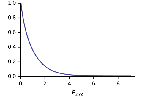
25. The curves approximate the normal distribution.
27. ten
29. SS = 237.33; MS = 23.73
31. 0.1614
33. two
35. SS = 5,700.4;, MS = 2,850.2
37. 3.6101
39. Yes, there is enough evidence to show that the scores among the groups are statistically significant at the 10% level.
Test of Two Variances – Practice
43. The populations from which the two samples are drawn are normally distributed.
45. H0: σ1 = σ2, Ha: σ1 < σ2, or, H0: σ21 = σ22, Ha: σ21<σ22
47. 4.11
49. 0.7159
51. No, at the 10% level of significance, we do not reject the null hypothesis and state that the data do not show that the variation in drive times for the first worker is less than the variation in drive times for the second worker.
53. 2.8674
55. Reject the null hypothesis. There is enough evidence to say that the variance of the grades for the first student is higher than the variance in the grades for the second student.
57. 0.7414
One-Way ANOVA – Homework
59. SSbetween = 26, SSwithin = 441, F = 0.2653
The F Distribution and the F-Ratio – Homework
62. df(denom) = 15
Facts About the F Distribution – Homework
64.
- H0: µL = µT = µJ
- at least any two of the means are different
- df(num) = 2; df(denom) = 12
- F distribution
- 0.67
- 0.5305
- Check student’s solution.
- Decision: Do not reject the null hypothesis; Conclusion: There is insufficient evidence to conclude that the means are different.
- Ha: µd = µn = µh
- At least any two of the magazines have different mean lengths.
- df(num) = 2, df(denom) = 12
- F distribtuion
- F = 15.28
- p-value = 0.001
- Check student’s solution.
- Alpha: 0.05
- Decision: Reject the Null Hypothesis.
- Reason for decision: p-value < alpha
- Conclusion: There is sufficient evidence to conclude that the mean lengths of the magazines are different.
69.
- H0: μo = μh = μf
- At least two of the means are different.
- df(n) = 2, df(d) = 13
- F2,13
- 0.64
- 0.5437
- Check student’s solution.
- Alpha: 0.05
- Decision: Do not reject the null hypothesis.
- Reason for decision: p-value > alpha
- Conclusion: The mean scores of different class delivery are not different.
71.
- H0: μp = μm = μh
- At least any two of the means are different.
- df(n) = 2, df(d) = 12
- F2,12
- 3.13
- 0.0807
- Check student’s solution.
- Alpha: 0.05
- Decision: Do not reject the null hypothesis.
- Reason for decision: p-value > alpha
- Conclusion: There is not sufficient evidence to conclude that the mean numbers of daily visitors are different.
73.
The data appear normally distributed from the chart and of a similar spread. There do not appear to be any serious outliers, so we may proceed with our ANOVA calculations, to see if we have good evidence of a difference between the three groups.
H0: μ1 = μ2 = μ3;
Ha: μi ≠ μj some i ≠ j.
Define μ1, μ2, μ3, as the population mean number of eggs laid by the three groups of fruit flies.
F statistic = 8.6657;
p-value = 0.0004
Decision: Since the p-value is less than the level of significance of 0.01, we reject the null hypothesis.
Conclusion: We have good evidence that the average number of eggs laid during the first 14 days of life for these three strains of fruitflies is different.
Interestingly, if you perform a two-sample t-test to compare the RS and NS groups they are significantly different (p = 0.0013). Similarly, SS and NS are significantly different (p = 0.0006). However, the two selected groups, RS and SS are not significantly different (p = 0.5176). Thus we appear to have good evidence that selection either for resistance or for susceptibility involves a reduced rate of egg production (for these specific strains) as compared to flies that were not selected for resistance or susceptibility to DDT. Here, genetic selection has apparently involved a loss of fecundity.
Test of Two Variances – Homework
75.
H0: σ21=σ22
Ha: σ21≠σ21
df(num) = 4; df(denom) = 4
F4, 4
3.00
2(0.1563) = 0.3126. Using the TI-83+/84+ function 2-SampFtest, you get the test statistic as 2.9986 and p-value directly as 0.3127. If you input the lists in a different order, you get a test statistic of 0.3335 but the p-value is the same because this is a two-tailed test.
Check student’t solution.
Decision: Do not reject the null hypothesis; Conclusion: There is insufficient evidence to conclude that the variances are different.
78. The answers may vary. Sample answer: Home decorating magazines and news magazines have different variances.
80.
- H0: = σ21 = σ22
- Ha: σ21 ≠ σ21
- df(n) = 7, df(d) = 6
- F7,6
- 0.8117
- 0.7825
- Check student’s solution.
- Alpha: 0.05
- Decision: Do not reject the null hypothesis.
- Reason for decision: p-value > alpha
- Conclusion: There is not sufficient evidence to conclude that the variances are different.
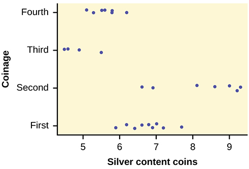
While there are differences in spread, it is not unreasonable to use ANOVA techniques. Here is the completed ANOVA table:
| Source of Variation | Sum of Squares (SS) | Degrees of Freedom (df) | Mean Square (MS) | F |
|---|---|---|---|---|
| Factor (Between) | 37.748 | 4 – 1 = 3 | 12.5825 | 26.272 |
| Error (Within) | 11.015 | 27 – 4 = 23 | 0.4789 | |
| Total | 48.763 | 27 – 1 = 26 |
P(F > 26.272) = 0;
Reject the null hypothesis for any alpha. There is sufficient evidence to conclude that the mean silver content among the four coinages is different. From the strip chart, it appears that the first and second coinages had higher silver contents than the third and fourth.
83.
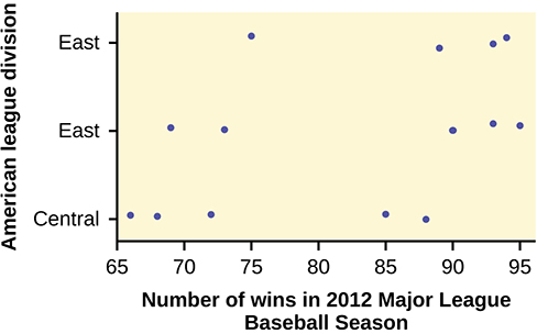
While the spread seems similar, there may be some question about the normality of the data, given the wide gaps in the middle near the 0.500 mark of 82 games (teams play 162 games each season in MLB). However, one-way ANOVA is robust.
Here is the ANOVA table for the data:
| Source of Variation | Sum of Squares (SS) | Degrees of Freedom (df) | Mean Square (MS) | F |
|---|---|---|---|---|
| Factor (Between) | 344.16 | 3 – 1 = 2 | 172.08 | 26.272 |
| Error (Within) | 1,219.55 | 14 – 3 = 11 | 110.87 | 1.5521 |
| Total | 1,563.71 | 14 – 1 = 13 |
P(F > 1.5521) = 0.2548
Since the p-value is so large, there is not good evidence against the null hypothesis of equal means. We decline to reject the null hypothesis. Thus, for 2012, there is not any have any good evidence of a significant difference in the mean number of wins between the divisions of the American League.
Candela Citations
- Introductory Statistics. Authored by: Barbara Illowsky, Susan Dean. Provided by: OpenStax. Located at: https://openstax.org/books/introductory-statistics/pages/1-introduction. License: CC BY: Attribution. License Terms: Access for free at https://openstax.org/books/introductory-statistics/pages/1-introduction