Learning Outcomes
- Describe the characteristics of a chi-square distribution
The notation for the chi-square distribution is:
[latex]\displaystyle\chi\sim\chi^2_{df}[/latex]
where df = degrees of freedom which depends on how chi-square is being used. (If you want to practice calculating chi-square probabilities then use [latex]\displaystyle{df}=n-1[/latex]. The degrees of freedom for the three major uses are each calculated differently).
For the χ2 distribution, the population mean is μ = df and the population standard deviation is [latex]\displaystyle\sigma=\sqrt{2(df)}[/latex].
The random variable is shown as χ2, but may be any upper case letter.
Recall: Skewness
In a perfectly symmetrical distribution, the mean and the median are the same. The histogram for the data: 4; 5; 6; 6; 6; 7; 7; 7; 7; 8 (shown in the Figure below) is not symmetrical. A distribution of this type is called skewed to the left because the majority of the data is around 6 or 7, the mean is going to be highly affected by a value further away from the middle, in this case, 4. In order words, the value to the left, 4, is pulling the mean in that direction.

The histogram for the data: 6; 7; 7; 7; 7; 8; 8; 8; 9; 10 (shown in the Figure below) is also not symmetrical. It is skewed to the right.

The mean is 7.7, the median is 7.5, and the mode is seven. The value to the right, 10, is pulling the mean in that direction. To summarize, generally, if the distribution of data is skewed to the left, the mean is less than the median, which is often less than the mode. If the distribution of data is skewed to the right, the mode is often less than the median, which is less than the mean.
The random variable for a chi-square distribution with k degrees of freedom is the sum of k independent, squared standard normal variables.
[latex]\displaystyle\chi^2=(Z_1)^2+(Z_2)^2+\dots+(Z_k)^2[/latex]
- The curve is nonsymmetrical and skewed to the right.
- There is a different chi-square curve for each df.
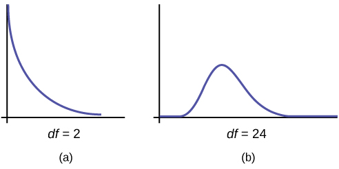
- The test statistic for any test is always greater than or equal to zero.
- When df > 90, the chi-square curve approximates the normal distribution. For [latex]\displaystyle{X}\sim\chi^2_{1,000}[/latex] the mean, [latex]\displaystyle\mu=df=1,000[/latex] and the standard deviation, [latex]\displaystyle\sigma=\sqrt{2(1,000)}[/latex]. Therefore, [latex]\displaystyle{X}\sim{N}(1,000, 44.7)[/latex], approximately.
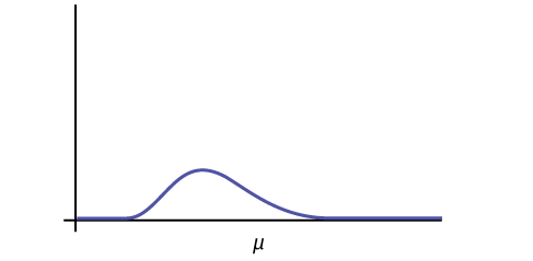
- The mean, μ, is located just to the right of the peak.
Candela Citations
- Introductory Statistics. Authored by: Barbara Illowsky, Susan Dean. Provided by: OpenStax. Located at: https://openstax.org/books/introductory-statistics/pages/1-introduction. License: CC BY: Attribution. License Terms: Access for free at https://openstax.org/books/introductory-statistics/pages/1-introduction