Learning Outcomes
- Given the mean of an exponential distribution, create a model for the distribution
- Calculate probabilities for an exponential distribution
- Calculate percentiles for an exponential distribution
Recall: Exponents
Exponents are used to represent repeated multiplication of the same number. For example,
[latex]x^3 = x \cdot x \cdot x[/latex]
so, multiplying [latex]x[/latex] by iteself [latex]3[/latex] times.

This is read [latex]a[/latex] to the [latex]{m}^{\mathrm{th}}[/latex] power.
Recall: [latex]e[/latex]
The letter e represents the irrational number
The letter e is used as a base for many real-world exponential models. To work with base e, we use the approximation, [latex]e\approx 2.718282[/latex]. The constant was named by the Swiss mathematician Leonhard Euler (1707–1783) who first investigated and discovered many of its properties.
The exponential distribution is often concerned with the amount of time until some specific event occurs. For example, the amount of time (beginning now) until an earthquake occurs has an exponential distribution. Other examples include the length, in minutes, of long distance business telephone calls, and the amount of time, in months, a car battery lasts. It can be shown, too, that the value of the change that you have in your pocket or purse approximately follows an exponential distribution.
Values for an exponential random variable occur in the following way. There are fewer large values and more small values. For example, the amount of money customers spend in one trip to the supermarket follows an exponential distribution. There are more people who spend small amounts of money and fewer people who spend large amounts of money.
The exponential distribution is widely used in the field of reliability. Reliability deals with the amount of time a product lasts.
Recall: Negative Exponents
The Negative Rule of Exponents
For any nonzero real number [latex]a[/latex] and natural number [latex]n[/latex], the negative rule of exponents states that
Example
Let X = amount of time (in minutes) a postal clerk spends with his or her customer. The time is known to have an exponential distribution with the average amount of time equal to four minutes.
X is a continuous random variable since time is measured. It is given that μ = 4 minutes. To do any calculations, you must know m, the decay parameter.
[latex]{m}=\frac{1}{\mu}[/latex]. Therefore, [latex]{m}=\frac{1}{4}={0.25}[/latex]
The standard deviation, σ, is the same as the mean. μ = σ
The distribution notation is X ~ Exp(m). Therefore, X ~ Exp(0.25).
The probability density function is f(x) = me–mx. The number e = 2.71828182846… It is a number that is used often in mathematics. Scientific calculators have the key “ex.” If you enter one for x, the calculator will display the value e.
The curve is:
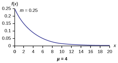
f(x) = 0.25e–0.25x where x is at least zero and m = 0.25.
For example, f(5) = 0.25e−(0.25)(5) = 0.072. The value 0.072 is the height of the curve when x = 5. Below, you will learn how to find probabilities using the decay parameter.
The graph is as follows:

Notice the graph is a declining curve. When x = 0, f(x) = 0.25e(−0.25)(0) = (0.25)(1) = 0.25 = m. The maximum value on the y-axis is m.
Try It
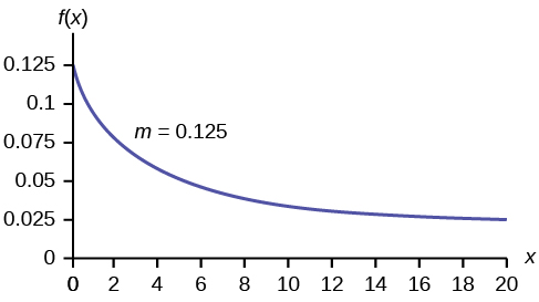
The amount of time spouses shop for anniversary cards can be modeled by an exponential distribution with the average amount of time equal to eight minutes. Write the distribution, state the probability density function, and graph the distribution.
Recall: Definition of the Natural Logarithm
A natural logarithm is a logarithm with base e. We write [latex]{\mathrm{log}}_{e}\left(x\right)[/latex] simply as [latex]\mathrm{ln}\left(x\right)[/latex]. The natural logarithm of a positive number x satisfies the following definition.
For [latex]x>0[/latex],
[latex]y=\mathrm{ln}\left(x\right)\text{ can be written as }{e}^{y}=x[/latex]
We read [latex]\mathrm{ln}\left(x\right)[/latex] as, “the logarithm with base e of x” or “the natural logarithm of x.”
The logarithm y is the exponent to which e must be raised to get x.
Since the functions [latex]y=e{}^{x}[/latex] and [latex]y=\mathrm{ln}\left(x\right)[/latex] are inverse functions, [latex]\mathrm{ln}\left({e}^{x}\right)=x[/latex] for all x and [latex]e{}^{\mathrm{ln}\left(x\right)}=x[/latex] for x > [latex]0[/latex].
Example
[latex]e^x=0.25[/latex]
[latex]ln(e^x)=ln(0.25)[/latex]
[latex]x \cdot ln(e)= ln(0.25)[/latex]
[latex]x=\frac{ln(0.25)}{ln(e)}[/latex]
[latex]x=\frac{-1.38629}{1}[/latex]
[latex]x=-1.38629[/latex]
Example
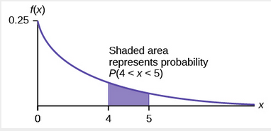
- Using the information in the previous Example, find the probability that a clerk spends four to five minutes with a randomly selected customer.
- Half of all customers are finished within how long? (Find the 50th percentile.)
- Which is larger, the mean or the median?
Try It
The number of days ahead travelers purchase their airline tickets can be modeled by an exponential distribution with the average amount of time equal to 15 days. Find the probability that a traveler will purchase a ticket fewer than ten days in advance. How many days do half of all travelers wait?
Activity
Have each class member count the change he or she has in his or her pocket or purse. Your instructor will record the amounts in dollars and cents. Construct a histogram of the data taken by the class. Use five intervals. Draw a smooth curve through the bars. The graph should look approximately exponential. Then calculate the mean.
Let X = the amount of money a student in your class has in his or her pocket or purse.
The distribution for X is approximately exponential with mean, μ = _______ and m = _______. The standard deviation, σ = ________.
Draw the appropriate exponential graph. You should label the x– and y–axes, the decay rate, and the mean. Shade the area that represents the probability that one student has less than $.40 in his or her pocket or purse. (Shade P(x < 0.40)).
Example
On the average, a certain computer part lasts ten years. The length of time the computer part lasts is exponentially distributed.
- What is the probability that a computer part lasts more than 7 years?
- On the average, how long would five computer parts last if they are used one after another?
- Eighty percent of computer parts last at most how long?
- What is the probability that a computer part lasts between nine and 11 years?
Try It
On average, a pair of running shoes can last 18 months if used every day. The length of time running shoes last is exponentially distributed. What is the probability that a pair of running shoes last more than 15 months? On average, how long would six pairs of running shoes last if they are used one after the other? Eighty percent of running shoes last at most how long if used every day?
Example
Suppose that the length of a phone call, in minutes, is an exponential random variable with decay parameter = 112. If another person arrives at a public telephone just before you, find the probability that you will have to wait more than five minutes. Let X = the length of a phone call, in minutes.
What is m, μ, and σ? The probability that you must wait more than five minutes is _______ .
Try It
Suppose that the distance, in miles, that people are willing to commute to work is an exponential random variable with a decay parameter [latex]\frac{1}{20}[/latex]. Let X = the distance people are willing to commute in miles. What is m, μ, and σ? What is the probability that a person is willing to commute more than 25 miles?
Example
The time spent waiting between events is often modeled using the exponential distribution. For example, suppose that an average of 30 customers per hour arrive at a store and the time between arrivals is exponentially distributed.
- On average, how many minutes elapse between two successive arrivals?
- When the store first opens, how long on average does it take for three customers to arrive?
- After a customer arrives, find the probability that it takes less than one minute for the next customer to arrive.
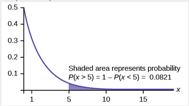
- After a customer arrives, find the probability that it takes more than five minutes for the next customer to arrive.
- Seventy percent of the customers arrive within how many minutes of the previous customer?
- Is an exponential distribution reasonable for this situation?
Try It
Suppose that on a certain stretch of highway, cars pass at an average rate of five cars per minute. Assume that the duration of time between successive cars follows the exponential distribution.
- On average, how many seconds elapse between two successive cars?
- After a car passes by, how long on average will it take for another seven cars to pass by?
- Find the probability that after a car passes by, the next car will pass within the next 20 seconds.
- Find the probability that after a car passes by, the next car will not pass for at least another 15 seconds.
Memorylessness of the Exponential Distribution
From the first Example, recall that the amount of time between customers is exponentially distributed with a mean of two minutes (X ~ Exp (0.5)). Suppose that five minutes have elapsed since the last customer arrived. Since an unusually long amount of time has now elapsed, it would seem to be more likely for a customer to arrive within the next minute. With the exponential distribution, this is not the case—the additional time spent waiting for the next customer does not depend on how much time has already elapsed since the last customer. This is referred to as the memoryless property. Specifically, the memoryless property says that
P (X > r + t | X > r) = P (X > t) for all r ≥ 0 and t ≥ 0
For example, if five minutes has elapsed since the last customer arrived, then the probability that more than one minute will elapse before the next customer arrives is computed by using r = 5 and t = 1 in the foregoing equation.
P(X > 5 + 1 | X > 5) = P(X > 1) = e(–0.5)(1) ≈ 0.6065.
This is the same probability as that of waiting more than one minute for a customer to arrive after the previous arrival.
The exponential distribution is often used to model the longevity of an electrical or mechanical device. In an earlier Example, the lifetime of a certain computer part has the exponential distribution with a mean of ten years (X ~ Exp(0.1)). The memoryless property says that knowledge of what has occurred in the past has no effect on future probabilities. In this case it means that an old part is not any more likely to break down at any particular time than a brand new part. In other words, the part stays as good as new until it suddenly breaks. For example, if the part has already lasted ten years, then the probability that it lasts another seven years is P(X > 17|X > 10) =P(X > 7) = 0.4966.
Example
Refer to the first Example, where the time a postal clerk spends with his or her customer has an exponential distribution with a mean of four minutes. Suppose a customer has spent four minutes with a postal clerk. What is the probability that he or she will spend at least an additional three minutes with the postal clerk?
The decay parameter of X is m = 14 = 0.25, so X ∼ Exp(0.25).
The cumulative distribution function is P(X < x) = 1 – e–0.25x. We want to find P(X > 7|X > 4). The memoryless property says that P(X > 7|X > 4) = P (X > 3), so we just need to find the probability that a customer spends more than three minutes with a postal clerk.
This is P(X > 3) = 1 – P (X < 3) = 1 – (1 – e–0.25⋅3) = e–0.75 ≈ 0.4724.
USING THE TI-83, 83+, 84, 84+ CALCULATOR
1–(1–e^(–0.25*3)) = e^(–0.25*3)
Try It
Suppose that the longevity of a light bulb is exponential with a mean lifetime of eight years. If a bulb has already lasted 12 years, find the probability that it will last a total of over 19 years.
Recall: Factorial
Factorial is the product of a whole number and the whole numbers that came before it (to the left) on a number line, excluding zero. For example:
[latex]4!=4 \cdot 3 \cdot 2 \cdot 1 = 24[/latex]
Relationship between the Poisson and the Exponential Distribution
There is an interesting relationship between the exponential distribution and the Poisson distribution. Suppose that the time that elapses between two successive events follows the exponential distribution with a mean of μ units of time. Also assume that these times are independent, meaning that the time between events is not affected by the times between previous events. If these assumptions hold, then the number of events per unit time follows a Poisson distribution with mean λ = 1/μ. Recall that if X has the Poisson distribution with mean λ, then [latex]P(X=k)=\frac{{\lambda}^{k}{e}^{-\lambda}}{k!}[/latex]. Conversely, if the number of events per unit time follows a Poisson distribution, then the amount of time between events follows the exponential distribution. (k! = k*(k-1*)(k–2)*(k-3)…3*2*1)
USING THE TI-83, 83+, 84, 84+ CALCULATOR
Suppose X has the Poisson distribution with mean λ. Compute P(X = k) by entering 2nd, VARS(DISTR), C: poissonpdf(λ, k). To compute P(X ≤ k), enter 2nd, VARS (DISTR), D:poissoncdf(λ, k).
Example
At a police station in a large city, calls come in at an average rate of four calls per minute. Assume that the time that elapses from one call to the next has the exponential distribution. Take note that we are concerned only with the rate at which calls come in, and we are ignoring the time spent on the phone. We must also assume that the times spent between calls are independent. This means that a particularly long delay between two calls does not mean that there will be a shorter waiting period for the next call. We may then deduce that the total number of calls received during a time period has the Poisson distribution.
- Find the average time between two successive calls.
- Find the probability that after a call is received, the next call occurs in less than ten seconds.
- Find the probability that exactly five calls occur within a minute.
- Find the probability that less than five calls occur within a minute.
- Find the probability that more than 40 calls occur in an eight-minute period.
Try It
In a small city, the number of automobile accidents occur with a Poisson distribution at an average of three per week.
- Calculate the probability that there are at most 2 accidents occur in any given week.
- What is the probability that there is at least two weeks between any 2 accidents?
Candela Citations
- OpenStax, The Exponential Distribution. Provided by: OpenStax. Located at: https://openstax.org/books/introductory-statistics/pages/5-3-the-exponential-distribution. License: CC BY: Attribution. License Terms: Access for free at https://openstax.org/books/introductory-statistics/pages/1-introduction
- Introductory Statistics. Authored by: Barbara Illowsky, Susan Dean. Provided by: Open Stax. Located at: https://openstax.org/books/introductory-statistics/pages/1-introduction. License: CC BY: Attribution. License Terms: Access for free at https://openstax.org/books/introductory-statistics/pages/1-introduction
- Unit 11: Exponents and Polynomials, from Developmental Math: An Open Program. Provided by: Monterey Institute of Technology and Education. Located at: http://nrocnetwork.org/resources/downloads/nroc-math-open-textbook-units-1-12-pdf-and-word-formats/. License: CC BY: Attribution
- Precalculus. Authored by: Jay Abramson, et al. Provided by: OpenStax. Located at: https://openstax.org/books/precalculus/pages/1-introduction-to-functions. License: CC BY: Attribution. License Terms: Access for free at https://openstax.org/books/precalculus/pages/1-introduction-to-functions
- Prealgebra. Provided by: OpenStax. Located at: https://openstax.org/books/prealgebra/pages/1-introduction. License: CC BY: Attribution. License Terms: Access for free at https://openstax.org/books/prealgebra/pages/1-introduction


