When we make an estimate for a population, how reliable is our estimate?
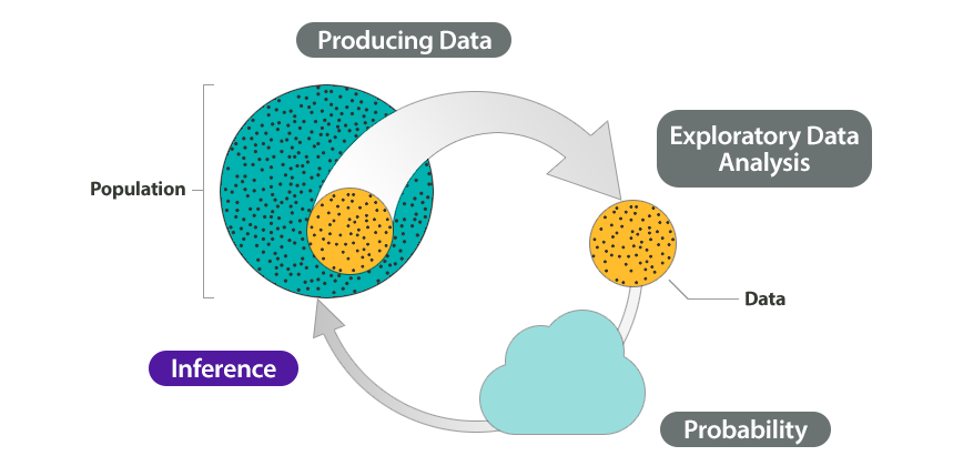
This module introduces us to one of the two big concepts involving inference – confidence intervals. First, let’s review the Big Picture of Statistics. In the Big Picture of Statistics, we use data from a sample to “infer” something about the population. Inference is based on probability.
Example
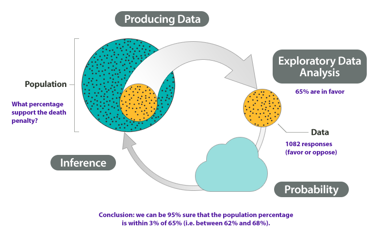
At the end of April 2005, ABC News and the Washington Post conducted a poll to determine the percentage of U.S. adults who support the death penalty.
Research question: What percentage of U.S. adults support the death penalty?
Steps in the statistical investigation:
- Produce Data: Determine what to measure, then collect the data. The poll selected 1,082 U.S. adults at random. Each adult answered this question: “Do you favor or oppose the death penalty for a person convicted of murder?”
- Explore the Data: Analyze and summarize the data. In the sample, 65% favored the death penalty.
- Draw a Conclusion: Use the data, probability, and statistical inference to draw a conclusion about the population.
Our goal is to determine the percentage of the U.S. adult population that support the death penalty. We know that different samples give different results. What are the chances that a sample reflects the opinions of the population within 3%? Probability describes the likelihood that a sample is this accurate, so we can say with 95% confidence that between 62% and 68% of the population favor the death penalty.
We illustrated the Big Picture of Statistics with an example about an inference made from survey data. From a random sample of U.S. adults, we estimated the percentage of all U.S. adults who support the death penalty. We saw that probability describes the likelihood that an estimate is within 3% of the true percentage with this opinion in the population. For this example, there is a 95% chance that a random sample is within 3% of the true population percentage.
The purpose of a confidence interval is to estimate a population parameter on the basis of a sample statistic. Sample statistics vary, so there is always error in our estimate, but we never know how much. We therefore use the standard error, which is the average error in our sample estimates, to create a margin of error. The margin of error is related to our confidence that the interval contains the population parameter.
Here we add these ideas to the Big Picture to show how probability connects to inference.
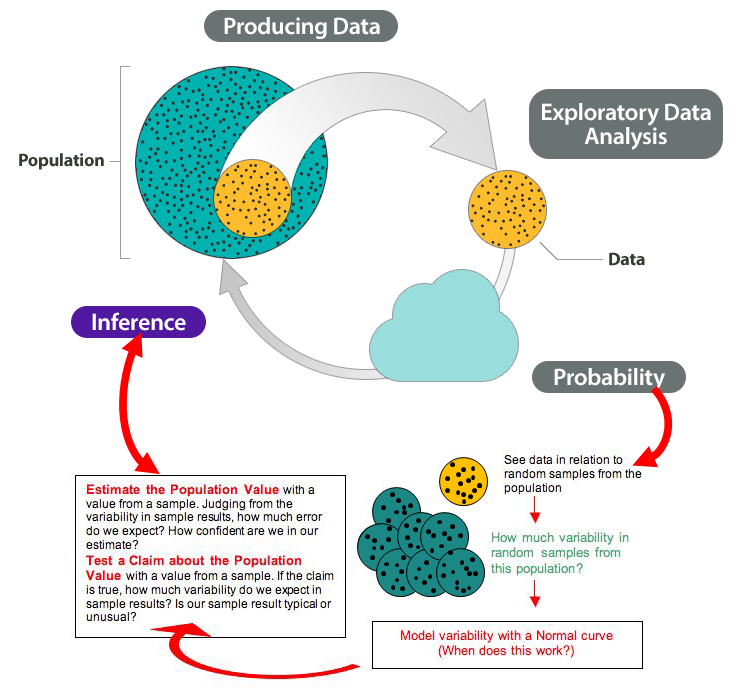
Note that we highlighted two types of inference in the diagram:
- Estimate a population value.
- Test a claim about the population value.
In the module Confidence Intervals, we will be focusing on estimating a single population proportion and a single population mean. In future modules, we will be testing claims about population values.
Candela Citations
- Provided by: Lumen Learning. License: All Rights Reserved
- Provided by: Lumen Learning. License: CC BY: Attribution
- Concepts in Statistics. Provided by: Open Learning Initiative. Located at: http://oli.cmu.edu. License: CC BY: Attribution