As we’ve learned, there are a multitude of situations that can be modeled by exponential functions, such as investment growth, radioactive decay, atmospheric pressure changes, and temperatures of a cooling object. What do these phenomena have in common? For one thing, all the models either increase or decrease as time moves forward. But that’s not the whole story. It’s the way data increase or decrease that helps us determine whether it is best modeled by an exponential equation. Knowing the behavior of exponential functions in general allows us to recognize when to use exponential regression, so let’s review exponential growth and decay.
Recall that exponential functions have the form [latex]y=a{b}^{x}[/latex] or [latex]y={A}_{0}{e}^{kx}[/latex]. When performing regression analysis, we use the form most commonly used on graphing utilities, [latex]y=a{b}^{x}[/latex]. Take a moment to reflect on the characteristics we’ve already learned about the exponential function [latex]y=a{b}^{x}[/latex] (assume a > 0):
- b must be greater than zero and not equal to one.
- The initial value of the model is y = a.
- If b > 1, the function models exponential growth. As x increases, the outputs of the model increase slowly at first, but then increase more and more rapidly, without bound.
- If 0 < b < 1, the function models exponential decay. As x increases, the outputs for the model decrease rapidly at first and then level off to become asymptotic to the x-axis. In other words, the outputs never become equal to or less than zero.
As part of the results, your calculator will display a number known as the correlation coefficient, labeled by the variable r, or [latex]{r}^{2}[/latex]. (You may have to change the calculator’s settings for these to be shown.) The values are an indication of the “goodness of fit” of the regression equation to the data. We more commonly use the value of [latex]{r}^{2}[/latex] instead of r, but the closer either value is to 1, the better the regression equation approximates the data.
A General Note: Exponential Regression
Exponential regression is used to model situations in which growth begins slowly and then accelerates rapidly without bound, or where decay begins rapidly and then slows down to get closer and closer to zero. We use the command “ExpReg” on a graphing utility to fit an exponential function to a set of data points. This returns an equation of the form, [latex]y=a{b}^{x}[/latex]
Note that:
- b must be non-negative.
- when b > 1, we have an exponential growth model.
- when 0 < b < 1, we have an exponential decay model.
How To: Given a set of data, perform exponential regression using a graphing utility.
- Use the STAT then EDIT menu to enter given data.
- Clear any existing data from the lists.
- List the input values in the L1 column.
- List the output values in the L2 column.
- Graph and observe a scatter plot of the data using the STATPLOT feature.
- Use ZOOM [9] to adjust axes to fit the data.
- Verify the data follow an exponential pattern.
- Find the equation that models the data.
- Select “ExpReg” from the STAT then CALC menu.
- Use the values returned for a and b to record the model, [latex]y=a{b}^{x}[/latex].
- Graph the model in the same window as the scatterplot to verify it is a good fit for the data.
Example 1: Using Exponential Regression to Fit a Model to Data
In 2007, a university study was published investigating the crash risk of alcohol impaired driving. Data from 2,871 crashes were used to measure the association of a person’s blood alcohol level (BAC) with the risk of being in an accident. The table below shows results from the study.[1] The relative risk is a measure of how many times more likely a person is to crash. So, for example, a person with a BAC of 0.09 is 3.54 times as likely to crash as a person who has not been drinking alcohol.
| BAC | 0 | 0.01 | 0.03 | 0.05 | 0.07 | 0.09 |
| Relative Risk of Crashing | 1 | 1.03 | 1.06 | 1.38 | 2.09 | 3.54 |
| BAC | 0.11 | 0.13 | 0.15 | 0.17 | 0.19 | 0.21 |
| Relative Risk of Crashing | 6.41 | 12.6 | 22.1 | 39.05 | 65.32 | 99.78 |
- Let x represent the BAC level, and let y represent the corresponding relative risk. Use exponential regression to fit a model to these data.
- After 6 drinks, a person weighing 160 pounds will have a BAC of about 0.16. How many times more likely is a person with this weight to crash if they drive after having a 6-pack of beer? Round to the nearest hundredth.
Solution
- Using the STAT then EDIT menu on a graphing utility, list the BAC values in L1 and the relative risk values in L2. Then use the STATPLOT feature to verify that the scatterplot follows the exponential pattern shown in Figure 1:
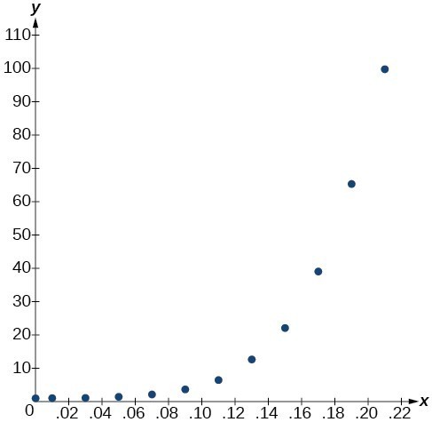
Figure 1
Use the “ExpReg” command from the STAT then CALC menu to obtain the exponential model,
[latex]y=0.58304829{\left(2.20720213\text{E}10\right)}^{x}[/latex]Converting from scientific notation, we have:
[latex]y=0.58304829{\left(\text{22,072,021,300}\right)}^{x}[/latex]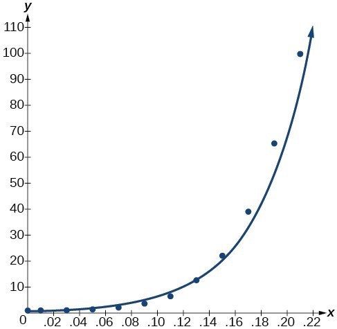
Figure 2
Notice that [latex]{r}^{2}\approx 0.97[/latex] which indicates the model is a good fit to the data. To see this, graph the model in the same window as the scatterplot to verify it is a good fit as shown in Figure 2:
-
Use the model to estimate the risk associated with a BAC of 0.16. Substitute 0.16 for x in the model and solve for y.
[latex]\begin{cases}y\hfill & =0.58304829{\left(\text{22,072,021,300}\right)}^{x}\hfill & \text{Use the regression model found in part (a)}\text{.}\hfill \\ \hfill & =0.58304829{\left(\text{22,072,021,300}\right)}^{0.16}\hfill & \text{Substitute 0}\text{.16 for }x\text{.}\hfill \\ \hfill & \approx \text{26}\text{.35}\hfill & \text{Round to the nearest hundredth}\text{.}\hfill \end{cases}[/latex]If a 160-pound person drives after having 6 drinks, he or she is about 26.35 times more likely to crash than if driving while sober.
Try It 1
The table below shows a recent graduate’s credit card balance each month after graduation.
| Month | 1 | 2 | 3 | 4 | 5 | 6 | 7 | 8 |
| Debt ($) | 620.00 | 761.88 | 899.80 | 1039.93 | 1270.63 | 1589.04 | 1851.31 | 2154.92 |
a. Use exponential regression to fit a model to these data.
b. If spending continues at this rate, what will the graduate’s credit card debt be one year after graduating?
Q & A
Is it reasonable to assume that an exponential regression model will represent a situation indefinitely?
No. Remember that models are formed by real-world data gathered for regression. It is usually reasonable to make estimates within the interval of original observation (interpolation). However, when a model is used to make predictions, it is important to use reasoning skills to determine whether the model makes sense for inputs far beyond the original observation interval (extrapolation).
Candela Citations
- Precalculus. Authored by: Jay Abramson, et al.. Provided by: OpenStax. Located at: http://cnx.org/contents/fd53eae1-fa23-47c7-bb1b-972349835c3c@5.175. License: CC BY: Attribution. License Terms: Download For Free at : http://cnx.org/contents/fd53eae1-fa23-47c7-bb1b-972349835c3c@5.175.
- Source: Indiana University Center for Studies of Law in Action, 2007 ↵