Identifying Local Behavior of Polynomial Functions
In addition to the end behavior of polynomial functions, we are also interested in what happens in the “middle” of the function. In particular, we are interested in locations where graph behavior changes. A turning point is a point at which the function values change from increasing to decreasing or decreasing to increasing.
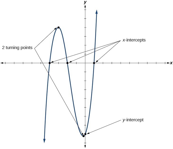
Figure 10
We are also interested in the intercepts. As with all functions, the y-intercept is the point at which the graph intersects the vertical axis. The point corresponds to the coordinate pair in which the input value is zero. Because a polynomial is a function, only one output value corresponds to each input value so there can be only one y-intercept [latex]\left(0,{a}_{0}\right).[/latex] The x-intercepts occur at the input values that correspond to an output value of zero. It is possible to have more than one x-intercept.
A General Note: Intercepts and Turning Points of Polynomial Functions
A turning point of a graph is a point at which the graph changes direction from increasing to decreasing or decreasing to increasing. The y-intercept is the point at which the function has an input value of zero. The x-intercepts are the points at which the output value is zero.
How To: Given a polynomial function, determine the intercepts.
- Determine the y-intercept by setting [latex]x=0[/latex] and finding the corresponding output value.
- Determine the x-intercepts by solving for the input values that yield an output value of zero.
Example 8: Determining the Intercepts of a Polynomial Function
Given the polynomial function [latex]f\left(x\right)=\left(x - 2\right)\left(x+1\right)\left(x - 4\right),\\[/latex] written in factored form for your convenience, determine the y– and x-intercepts.
Solution
The y-intercept occurs when the input is zero so substitute 0 for x.
The y-intercept is (0, 8).
The x-intercepts occur when the output is zero.
The x-intercepts are
[latex]\left(2,0\right),\left(-1,0\right), \text{and} \left(4,0\right).\\[/latex]
We can see these intercepts on the graph of the function shown in Figure 11.
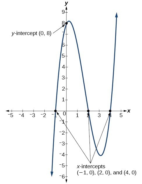
Figure 11
Example 9: Determining the Intercepts of a Polynomial Function with Factoring
Given the polynomial function [latex]f\left(x\right)={x}^{4}-4{x}^{2}-45,\\[/latex] determine the y– and x-intercepts.
Solution
The y-intercept occurs when the input is zero.
The y-intercept is [latex]\left(0,-45\right).[/latex]
The x-intercepts occur when the output is zero. To determine when the output is zero, we will need to factor the polynomial.
The x-intercepts are [latex]\left(3,0\right) \text{and} \left(-3,0\right).[/latex]
We can see these intercepts on the graph of the function shown in Figure 12. We can see that the function is even because [latex]f\left(x\right)=f\left(-x\right).\\[/latex]
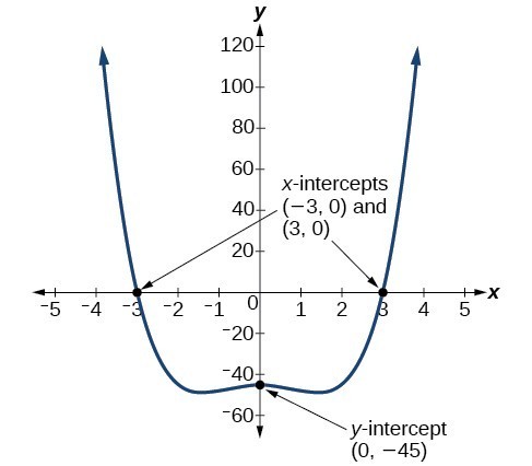
Figure 12
Try It 6
Given the polynomial function [latex]f\left(x\right)=2{x}^{3}-6{x}^{2}-20x,\\[/latex] determine the y– and x-intercepts.
Comparing Smooth and Continuous Graphs
The degree of a polynomial function helps us to determine the number of x-intercepts and the number of turning points. A polynomial function of nth degree is the product of n factors, so it will have at most n roots or zeros, or x-intercepts. The graph of the polynomial function of degree n must have at most n – 1 turning points. This means the graph has at most one fewer turning point than the degree of the polynomial or one fewer than the number of factors.
A continuous function has no breaks in its graph: the graph can be drawn without lifting the pen from the paper. A smooth curve is a graph that has no sharp corners. The turning points of a smooth graph must always occur at rounded curves. The graphs of polynomial functions are both continuous and smooth.
A General Note: Intercepts and Turning Points of Polynomials
A polynomial of degree n will have, at most, n x-intercepts and n – 1 turning points.
Example 10: Determining the Number of Intercepts and Turning Points of a Polynomial
Without graphing the function, determine the local behavior of the function by finding the maximum number of x-intercepts and turning points for [latex]f\left(x\right)=-3{x}^{10}+4{x}^{7}-{x}^{4}+2{x}^{3}.\\[/latex]
Solution
The polynomial has a degree of 10, so there are at most n x-intercepts and at most n – 1 turning points.
Try It 7
Without graphing the function, determine the maximum number of x-intercepts and turning points for [latex]f\left(x\right)=108 - 13{x}^{9}-8{x}^{4}+14{x}^{12}+2{x}^{3}\\[/latex]
Example 11: Drawing Conclusions about a Polynomial Function from the Graph
What can we conclude about the polynomial represented by the graph shown in the graph in Figure 13 based on its intercepts and turning points?
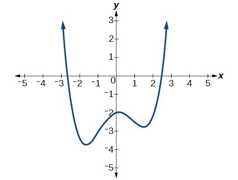
Figure 13
Solution
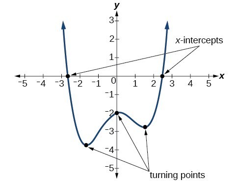
Figure 14
The end behavior of the graph tells us this is the graph of an even-degree polynomial.
The graph has 2 x-intercepts, suggesting a degree of 2 or greater, and 3 turning points, suggesting a degree of 4 or greater. Based on this, it would be reasonable to conclude that the degree is even and at least 4.
Try It 8
What can we conclude about the polynomial represented by Figure 15 based on its intercepts and turning points?
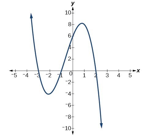
Figure 15
Example 12: Drawing Conclusions about a Polynomial Function from the Factors
Given the function [latex]f\left(x\right)=-4x\left(x+3\right)\left(x - 4\right),\\[/latex] determine the local behavior.
Solution
The y-intercept is found by evaluating [latex]f\left(0\right).[/latex]
The y-intercept is [latex]\left(0,0\right).[/latex]
The x-intercepts are found by determining the zeros of the function.
The x-intercepts are [latex]\left(0,0\right),\left(-3,0\right) \text{and} \left(4,0\right).[/latex]
The degree is 3 so the graph has at most 2 turning points.
Try It 9
Given the function [latex]f\left(x\right)=0.2\left(x - 2\right)\left(x+1\right)\left(x - 5\right),\\[/latex] determine the local behavior.