Before we begin graphing, it is helpful to review the behavior of exponential growth. Recall the table of values for a function of the form [latex]f\left(x\right)={b}^{x}[/latex] whose base is greater than one. We’ll use the function [latex]f\left(x\right)={2}^{x}[/latex]. Observe how the output values in the table below change as the input increases by 1.
| x | –3 | –2 | –1 | 0 | 1 | 2 | 3 |
| [latex]f\left(x\right)={2}^{x}[/latex] | [latex]\frac{1}{8}[/latex] | [latex]\frac{1}{4}[/latex] | [latex]\frac{1}{2}[/latex] | 1 | 2 | 4 | 8 |
Each output value is the product of the previous output and the base, 2. We call the base 2 the constant ratio. In fact, for any exponential function with the form [latex]f\left(x\right)=a{b}^{x}[/latex], b is the constant ratio of the function. This means that as the input increases by 1, the output value will be the product of the base and the previous output, regardless of the value of a.
Notice from the table that
- the output values are positive for all values of x;
- as x increases, the output values increase without bound; and
- as x decreases, the output values grow smaller, approaching zero.
Figure 1 shows the exponential growth function [latex]f\left(x\right)={2}^{x}[/latex].
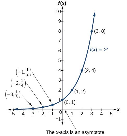
Figure 1. Notice that the graph gets close to the x-axis, but never touches it.
The domain of [latex]f\left(x\right)={2}^{x}[/latex] is all real numbers, the range is [latex]\left(0,\infty \right)[/latex], and the horizontal asymptote is [latex]y=0[/latex].
To get a sense of the behavior of exponential decay, we can create a table of values for a function of the form [latex]f\left(x\right)={b}^{x}[/latex] whose base is between zero and one. We’ll use the function [latex]g\left(x\right)={\left(\frac{1}{2}\right)}^{x}[/latex]. Observe how the output values in the table below change as the input increases by 1.
| x | –3 | –2 | –1 | 0 | 1 | 2 | 3 |
| [latex]g\left(x\right)=\left(\frac{1}{2}\right)^{x}[/latex] | 8 | 4 | 2 | 1 | [latex]\frac{1}{2}[/latex] | [latex]\frac{1}{4}[/latex] | [latex]\frac{1}{8}[/latex] |
Again, because the input is increasing by 1, each output value is the product of the previous output and the base, or constant ratio [latex]\frac{1}{2}[/latex].
Notice from the table that
- the output values are positive for all values of x;
- as x increases, the output values grow smaller, approaching zero; and
- as x decreases, the output values grow without bound.
The graph shows the exponential decay function, [latex]g\left(x\right)={\left(\frac{1}{2}\right)}^{x}[/latex].
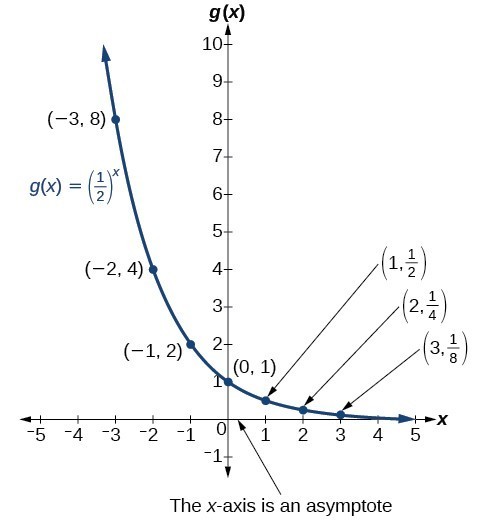
Figure 2. The domain of [latex]g\left(x\right)={\left(\frac{1}{2}\right)}^{x}[/latex] is all real numbers, the range is [latex]\left(0,\infty \right)[/latex], and the horizontal asymptote is [latex]y=0[/latex].
A General Note: Characteristics of the Graph of the Parent Function f(x) = bx
An exponential function with the form [latex]f\left(x\right)={b}^{x}[/latex], [latex]b>0[/latex], [latex]b\ne 1[/latex], has these characteristics:
- one-to-one function
- horizontal asymptote: [latex]y=0[/latex]
- domain: [latex]\left(-\infty , \infty \right)[/latex]
- range: [latex]\left(0,\infty \right)[/latex]
- x-intercept: none
- y-intercept: [latex]\left(0,1\right)[/latex]
- increasing if [latex]b>1[/latex]
- decreasing if [latex]b<1[/latex]
Compare the graphs of exponential growth and decay functions.
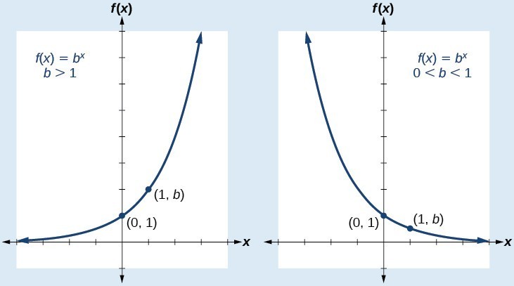
Figure 3
How To: Given an exponential function of the form [latex]f\left(x\right)={b}^{x}[/latex], graph the function.
- Create a table of points.
- Plot at least 3 point from the table, including the y-intercept [latex]\left(0,1\right)[/latex].
- Draw a smooth curve through the points.
- State the domain, [latex]\left(-\infty ,\infty \right)[/latex], the range, [latex]\left(0,\infty \right)[/latex], and the horizontal asymptote, [latex]y=0[/latex].
Example 1: Sketching the Graph of an Exponential Function of the Form f(x) = bx
Sketch a graph of [latex]f\left(x\right)={0.25}^{x}[/latex]. State the domain, range, and asymptote.
Solution
Before graphing, identify the behavior and create a table of points for the graph.
- Since b = 0.25 is between zero and one, we know the function is decreasing. The left tail of the graph will increase without bound, and the right tail will approach the asymptote y = 0.
- Create a table of points.
x –3 –2 –1 0 1 2 3 [latex]f\left(x\right)={0.25}^{x}[/latex] 64 16 4 1 0.25 0.0625 0.015625 - Plot the y-intercept, [latex]\left(0,1\right)[/latex], along with two other points. We can use [latex]\left(-1,4\right)[/latex] and [latex]\left(1,0.25\right)[/latex].
Draw a smooth curve connecting the points.
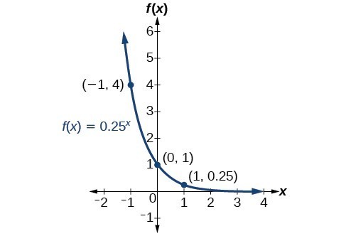
Figure 4. The domain is [latex]\left(-\infty ,\infty \right)[/latex]; the range is [latex]\left(0,\infty \right)[/latex]; the horizontal asymptote is [latex]y=0[/latex].
Try It 1
Sketch the graph of [latex]f\left(x\right)={4}^{x}[/latex]. State the domain, range, and asymptote.
Candela Citations
- Precalculus. Authored by: Jay Abramson, et al.. Provided by: OpenStax. Located at: http://cnx.org/contents/fd53eae1-fa23-47c7-bb1b-972349835c3c@5.175. License: CC BY: Attribution. License Terms: Download For Free at : http://cnx.org/contents/fd53eae1-fa23-47c7-bb1b-972349835c3c@5.175.