In real-world applications, we need to model the behavior of a function. In mathematical modeling, we choose a familiar general function with properties that suggest that it will model the real-world phenomenon we wish to analyze. In the case of rapid growth, we may choose the exponential growth function:
where [latex]{A}_{0}[/latex] is equal to the value at time zero, e is Euler’s constant, and k is a positive constant that determines the rate (percentage) of growth. We may use the exponential growth function in applications involving doubling time, the time it takes for a quantity to double. Such phenomena as wildlife populations, financial investments, biological samples, and natural resources may exhibit growth based on a doubling time. In some applications, however, as we will see when we discuss the logistic equation, the logistic model sometimes fits the data better than the exponential model.
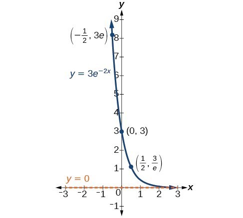
On the other hand, if a quantity is falling rapidly toward zero, without ever reaching zero, then we should probably choose the exponential decay model. Again, we have the form [latex]y={A}_{0}{e}^{kt}[/latex] where [latex]{A}_{0}[/latex] is the starting value, and e is Euler’s constant. Now k is a negative constant that determines the rate of decay. We may use the exponential decay model when we are calculating half-life, or the time it takes for a substance to exponentially decay to half of its original quantity. We use half-life in applications involving radioactive isotopes.
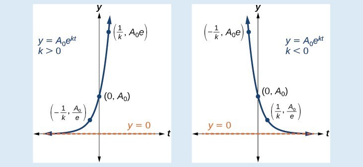
In our choice of a function to serve as a mathematical model, we often use data points gathered by careful observation and measurement to construct points on a graph and hope we can recognize the shape of the graph. Exponential growth and decay graphs have a distinctive shape, as we can see in Figure 2 and Figure 3. It is important to remember that, although parts of each of the two graphs seem to lie on the x-axis, they are really a tiny distance above the x-axis.

Exponential growth and decay often involve very large or very small numbers. To describe these numbers, we often use orders of magnitude. The order of magnitude is the power of ten, when the number is expressed in scientific notation, with one digit to the left of the decimal. For example, the distance to the nearest star, Proxima Centauri, measured in kilometers, is 40,113,497,200,000 kilometers. Expressed in scientific notation, this is [latex]4.01134972\times {10}^{13}[/latex]. So, we could describe this number as having order of magnitude [latex]{10}^{13}[/latex].
A General Note: Characteristics of the Exponential Function, [latex]y=A_{0}e^{kt}[/latex]
An exponential function with the form [latex]y={A}_{0}{e}^{kt}[/latex] has the following characteristics:
- one-to-one function
- horizontal asymptote: y = 0
- domain: [latex]\left(-\infty , \infty \right)[/latex]
- range: [latex]\left(0,\infty \right)[/latex]
- x intercept: none
- y-intercept: [latex]\left(0,{A}_{0}\right)[/latex]
- increasing if k > 0
- decreasing if k < 0
Example 1: Graphing Exponential Growth
A population of bacteria doubles every hour. If the culture started with 10 bacteria, graph the population as a function of time.
Solution
When an amount grows at a fixed percent per unit time, the growth is exponential. To find [latex]{A}_{0}[/latex] we use the fact that [latex]{A}_{0}[/latex] is the amount at time zero, so [latex]{A}_{0}=10[/latex]. To find k, use the fact that after one hour [latex]\left(t=1\right)[/latex] the population doubles from 10 to 20. The formula is derived as follows
so [latex]k=\mathrm{ln}\left(2\right)[/latex]. Thus the equation we want to graph is [latex]y=10{e}^{\left(\mathrm{ln}2\right)t}=10{\left({e}^{\mathrm{ln}2}\right)}^{t}=10\cdot {2}^{t}[/latex]. The graph is shown in Figure 5.
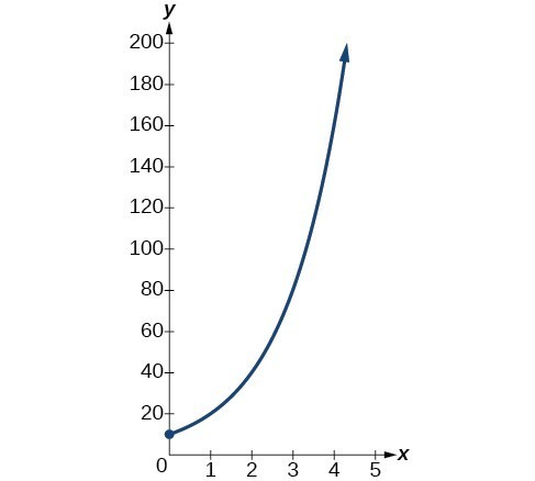
Figure 5. The graph of [latex]y=10{e}^{\left(\mathrm{ln}2\right)t}[/latex]
Half-Life
We now turn to exponential decay. One of the common terms associated with exponential decay, as stated above, is half-life, the length of time it takes an exponentially decaying quantity to decrease to half its original amount. Every radioactive isotope has a half-life, and the process describing the exponential decay of an isotope is called radioactive decay.
To find the half-life of a function describing exponential decay, solve the following equation:
We find that the half-life depends only on the constant k and not on the starting quantity [latex]{A}_{0}[/latex].
The formula is derived as follows
Since t, the time, is positive, k must, as expected, be negative. This gives us the half-life formula
How To: Given the half-life, find the decay rate.
- Write [latex]A={A}_{o}{e}^{kt}[/latex].
- Replace A by [latex]\frac{1}{2}{A}_{0}[/latex] and replace t by the given half-life.
- Solve to find k. Express k as an exact value (do not round).
Note: It is also possible to find the decay rate using [latex]k=-\frac{\mathrm{ln}\left(2\right)}{t}[/latex].
Example 2: Finding the Function that Describes Radioactive Decay
The half-life of carbon-14 is 5,730 years. Express the amount of carbon-14 remaining as a function of time, t.
Solution
This formula is derived as follows.
The function that describes this continuous decay is [latex]f\left(t\right)={A}_{0}{e}^{\left(\frac{\mathrm{ln}\left(0.5\right)}{5730}\right)t}[/latex]. We observe that the coefficient of t, [latex]\frac{\mathrm{ln}\left(0.5\right)}{5730}\approx -1.2097[/latex] is negative, as expected in the case of exponential decay.
Try It 1
The half-life of plutonium-244 is 80,000,000 years. Find function gives the amount of carbon-14 remaining as a function of time, measured in years.
Radiocarbon Dating
The formula for radioactive decay is important in radiocarbon dating, which is used to calculate the approximate date a plant or animal died. Radiocarbon dating was discovered in 1949 by Willard Libby, who won a Nobel Prize for his discovery. It compares the difference between the ratio of two isotopes of carbon in an organic artifact or fossil to the ratio of those two isotopes in the air. It is believed to be accurate to within about 1% error for plants or animals that died within the last 60,000 years.
Carbon-14 is a radioactive isotope of carbon that has a half-life of 5,730 years. It occurs in small quantities in the carbon dioxide in the air we breathe. Most of the carbon on Earth is carbon-12, which has an atomic weight of 12 and is not radioactive. Scientists have determined the ratio of carbon-14 to carbon-12 in the air for the last 60,000 years, using tree rings and other organic samples of known dates—although the ratio has changed slightly over the centuries.
As long as a plant or animal is alive, the ratio of the two isotopes of carbon in its body is close to the ratio in the atmosphere. When it dies, the carbon-14 in its body decays and is not replaced. By comparing the ratio of carbon-14 to carbon-12 in a decaying sample to the known ratio in the atmosphere, the date the plant or animal died can be approximated.
Since the half-life of carbon-14 is 5,730 years, the formula for the amount of carbon-14 remaining after t years is
where
- A is the amount of carbon-14 remaining
- [latex]{A}_{0}[/latex] is the amount of carbon-14 when the plant or animal began decaying.
This formula is derived as follows:
To find the age of an object, we solve this equation for t:
Out of necessity, we neglect here the many details that a scientist takes into consideration when doing carbon-14 dating, and we only look at the basic formula. The ratio of carbon-14 to carbon-12 in the atmosphere is approximately 0.0000000001%. Let r be the ratio of carbon-14 to carbon-12 in the organic artifact or fossil to be dated, determined by a method called liquid scintillation. From the equation [latex]A\approx {A}_{0}{e}^{-0.000121t}[/latex] we know the ratio of the percentage of carbon-14 in the object we are dating to the percentage of carbon-14 in the atmosphere is [latex]r=\frac{A}{{A}_{0}}\approx {e}^{-0.000121t}[/latex]. We solve this equation for t, to get
How To: Given the percentage of carbon-14 in an object, determine its age.
- Express the given percentage of carbon-14 as an equivalent decimal, k.
- Substitute for k in the equation [latex]t=\frac{\mathrm{ln}\left(r\right)}{-0.000121}[/latex] and solve for the age, t.
Example 2: Finding the Age of a Bone
A bone fragment is found that contains 20% of its original carbon-14. To the nearest year, how old is the bone?
Solution
We substitute 20% = 0.20 for k in the equation and solve for t:
The bone fragment is about 13,301 years old.
Analysis of the Solution
The instruments that measure the percentage of carbon-14 are extremely sensitive and, as we mention above, a scientist will need to do much more work than we did in order to be satisfied. Even so, carbon dating is only accurate to about 1%, so this age should be given as [latex]\text{13,301 years}\pm \text{1% or 13,301 years}\pm \text{133 years}[/latex].
Try It 2
Cesium-137 has a half-life of about 30 years. If we begin with 200 mg of cesium-137, will it take more or less than 230 years until only 1 milligram remains?
Calculating Doubling Time
For decaying quantities, we determined how long it took for half of a substance to decay. For growing quantities, we might want to find out how long it takes for a quantity to double. As we mentioned above, the time it takes for a quantity to double is called the doubling time.
Given the basic exponential growth equation [latex]A={A}_{0}{e}^{kt}[/latex], doubling time can be found by solving for when the original quantity has doubled, that is, by solving [latex]2{A}_{0}={A}_{0}{e}^{kt}[/latex].
The formula is derived as follows:
Thus the doubling time is
Example 3: Finding a Function That Describes Exponential Growth
According to Moore’s Law, the doubling time for the number of transistors that can be put on a computer chip is approximately two years. Give a function that describes this behavior.
Solution
The formula is derived as follows:
The function is [latex]A={A}_{0}{e}^{\frac{\mathrm{ln}2}{2}t}[/latex].
Try It 3
Recent data suggests that, as of 2013, the rate of growth predicted by Moore’s Law no longer holds. Growth has slowed to a doubling time of approximately three years. Find the new function that takes that longer doubling time into account.
Candela Citations
- Precalculus. Authored by: Jay Abramson, et al.. Provided by: OpenStax. Located at: http://cnx.org/contents/fd53eae1-fa23-47c7-bb1b-972349835c3c@5.175. License: CC BY: Attribution. License Terms: Download For Free at : http://cnx.org/contents/fd53eae1-fa23-47c7-bb1b-972349835c3c@5.175.
Analysis of the Solution
The population of bacteria after ten hours is 10,240. We could describe this amount is being of the order of magnitude [latex]{10}^{4}[/latex]. The population of bacteria after twenty hours is 10,485,760 which is of the order of magnitude [latex]{10}^{7}[/latex], so we could say that the population has increased by three orders of magnitude in ten hours.