Solutions to Try Its
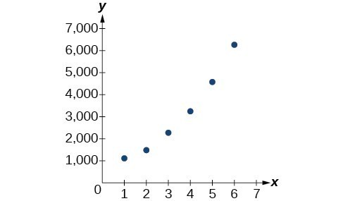
1. a. The exponential regression model that fits these data is [latex]y=522.88585984{\left(1.19645256\right)}^{x}[/latex].
b. If spending continues at this rate, the graduate’s credit card debt will be $4,499.38 after one year.
2. a. The logarithmic regression model that fits these data is [latex]y=141.91242949+10.45366573\mathrm{ln}\left(x\right)[/latex]
b. If sales continue at this rate, about 171,000 games will be sold in the year 2015.
3. a. The logistic regression model that fits these data is [latex]y=\frac{25.65665979}{1+6.113686306{e}^{-0.3852149008x}}[/latex].
b. If the population continues to grow at this rate, there will be about 25,634 seals in 2020.
c. To the nearest whole number, the carrying capacity is 25,657.
Solutions to Odd-Numbered Exercises
1. Logistic models are best used for situations that have limited values. For example, populations cannot grow indefinitely since resources such as food, water, and space are limited, so a logistic model best describes populations.
3. Regression analysis is the process of finding an equation that best fits a given set of data points. To perform a regression analysis on a graphing utility, first list the given points using the STAT then EDIT menu. Next graph the scatter plot using the STAT PLOT feature. The shape of the data points on the scatter graph can help determine which regression feature to use. Once this is determined, select the appropriate regression analysis command from the STAT then CALC menu.
5. The y-intercept on the graph of a logistic equation corresponds to the initial population for the population model.
7. C
9. B
11. [latex]P\left(0\right)=22[/latex] ; 175
13. [latex]p\approx 2.67[/latex]
15. y-intercept: [latex]\left(0,15\right)[/latex]
17. 4 koi
19.

21. 10 wolves
23. about 5.4 years.
25.
27. [latex]f\left(x\right)=776.682{e}^{0.3549x}[/latex]
29. When [latex]f\left(x\right)=4000[/latex], [latex]x\approx 4.6[/latex].
31. [latex]f\left(x\right)=731.92{\left(0.738\right)}^{x}[/latex]
33.
35.
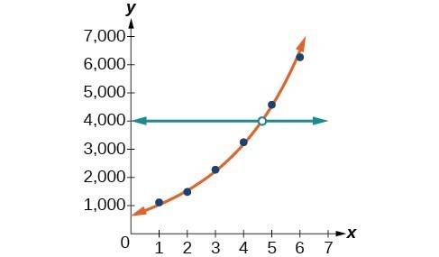
37. [latex]f\left(10\right)\approx 9.5[/latex]
39. When [latex]f\left(x\right)=7[/latex], [latex]x\approx 2.7[/latex].
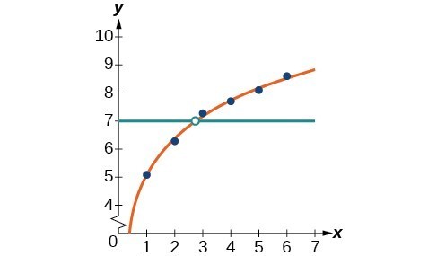
41. [latex]f\left(x\right)=7.544 - 2.268\mathrm{ln}\left(x\right)[/latex]
43.
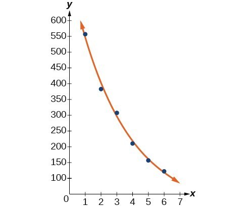
45.
47.

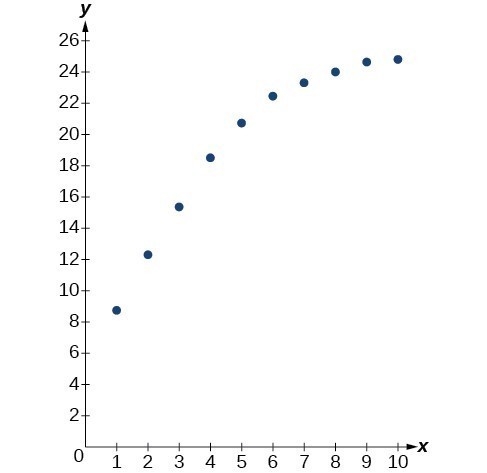
49. When [latex]f\left(x\right)=12.5[/latex], [latex]x\approx 2.1[/latex].

51. [latex]f\left(x\right)=\frac{136.068}{1+10.324{e}^{-0.480x}}[/latex]
53. about 136
55. Working with the left side of the equation, we see that it can be rewritten as [latex]a{e}^{-bt}[/latex]:
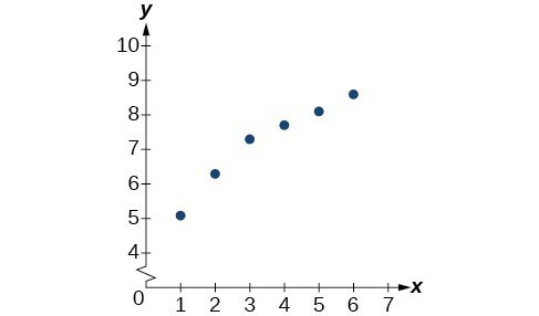
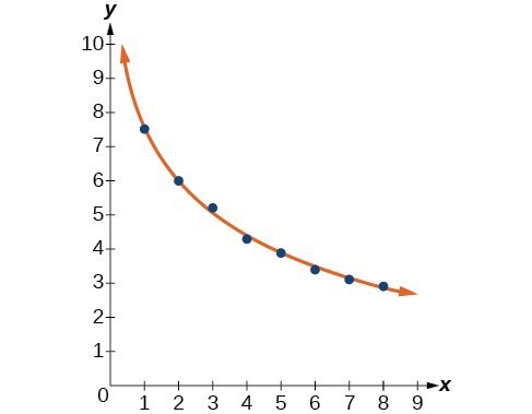
57. [latex]\frac{c-{P}_{0}}{{P}_{0}}{e}^{-bt}=\frac{c-\frac{c}{1+a}}{\frac{c}{1+a}}{e}^{-bt}=\frac{\frac{c\left(1+a\right)-c}{1+a}}{\frac{c}{1+a}}{e}^{-bt}=\frac{\frac{c\left(1+a - 1\right)}{1+a}}{\frac{c}{1+a}}{e}^{-bt}=\left(1+a - 1\right){e}^{-bt}=a{e}^{-bt}[/latex]
Thus, [latex]\frac{c-P\left(t\right)}{P\left(t\right)}=\frac{c-{P}_{0}}{{P}_{0}}{e}^{-bt}[/latex].
59. First rewrite the exponential with base e: [latex]f\left(x\right)=1.034341{e}^{0.247800x}[/latex]. Then test to verify that [latex]f\left(g\left(x\right)\right)=x[/latex], taking rounding error into consideration:
[latex]\begin{cases}g\left(f\left(x\right)\right)\hfill & =4.035510\mathrm{ln}\left(1.034341{e}^{\text{0}\text{.247800x}}\right)-0.136259\hfill \\ \hfill & =4.03551\left(\mathrm{ln}\left(1.034341\right)+\mathrm{ln}\left({e}^{\text{0}\text{.2478}x}\right)\right)-0.136259\hfill \\ \hfill & =4.03551\left(\mathrm{ln}\left(1.034341\right)+\text{0}\text{.2478}x\right)-0.136259\hfill \\ \hfill & =0.136257+0.999999x - 0.136259\hfill \\ \hfill & =-0.000002+0.999999x\hfill \\ \hfill & \approx 0+x\hfill \\ \hfill & =x\hfill \end{cases}[/latex]
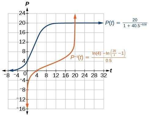
61. The graph of [latex]P\left(t\right)[/latex] has a y-intercept at (0, 4) and horizontal asymptotes at y = 0 and y = 20. The graph of [latex]{P}^{-1}\left(t\right)[/latex] has an x– intercept at (4, 0) and vertical asymptotes at x = 0 and x = 20.
Candela Citations
- Precalculus. Authored by: Jay Abramson, et al.. Provided by: OpenStax. Located at: http://cnx.org/contents/fd53eae1-fa23-47c7-bb1b-972349835c3c@5.175. License: CC BY: Attribution. License Terms: Download For Free at : http://cnx.org/contents/fd53eae1-fa23-47c7-bb1b-972349835c3c@5.175.