In the example above, Nicole’s earnings can be found by multiplying her sales by her commission. The formula e = 0.16s tells us her earnings, e, come from the product of 0.16, her commission, and the sale price of the vehicle. If we create a table, we observe that as the sales price increases, the earnings increase as well, which should be intuitive.
| s, sales prices | e = 0.16s | Interpretation |
|---|---|---|
| $4,600 | e = 0.16(4,600) = 736 | A sale of a $4,600 vehicle results in $736 earnings. |
| $9,200 | e = 0.16(9,200) = 1,472 | A sale of a $9,200 vehicle results in $1472 earnings. |
| $18,400 | e = 0.16(18,400) = 2,944 | A sale of a $18,400 vehicle results in $2944 earnings. |
Notice that earnings are a multiple of sales. As sales increase, earnings increase in a predictable way. Double the sales of the vehicle from $4,600 to $9,200, and we double the earnings from $736 to $1,472. As the input increases, the output increases as a multiple of the input. A relationship in which one quantity is a constant multiplied by another quantity is called direct variation. Each variable in this type of relationship varies directly with the other.
The graph below represents the data for Nicole’s potential earnings. We say that earnings vary directly with the sales price of the car. The formula [latex]y=k{x}^{n}[/latex] is used for direct variation. The value k is a nonzero constant greater than zero and is called the constant of variation. In this case, k = 0.16 and n = 1.
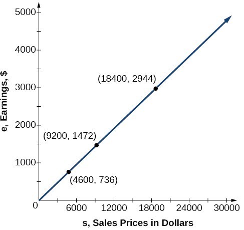
Figure 1
A General Note: Direct Variation
If x and y are related by an equation of the form
then we say that the relationship is direct variation and y varies directly with the nth power of x. In direct variation relationships, there is a nonzero constant ratio [latex]k=\frac{y}{{x}^{n}}[/latex], where k is called the constant of variation, which help defines the relationship between the variables.
How To: Given a description of a direct variation problem, solve for an unknown.
- Identify the input, x, and the output, y.
- Determine the constant of variation. You may need to divide y by the specified power of x to determine the constant of variation.
- Use the constant of variation to write an equation for the relationship.
- Substitute known values into the equation to find the unknown.
Example 1: Solving a Direct Variation Problem
The quantity y varies directly with the cube of x. If y = 25 when x = 2, find y when x is 6.
Solution
The general formula for direct variation with a cube is [latex]y=k{x}^{3}[/latex]. The constant can be found by dividing y by the cube of x.
Now use the constant to write an equation that represents this relationship.
Substitute x = 6 and solve for y.
Q & A
Do the graphs of all direct variation equations look like Example 1?
No. Direct variation equations are power functions—they may be linear, quadratic, cubic, quartic, radical, etc. But all of the graphs pass through (0, 0).
Try It 1
The quantity y varies directly with the square of x. If y = 24 when x = 3, find y when x is 4.
Candela Citations
- Precalculus. Authored by: Jay Abramson, et al.. Provided by: OpenStax. Located at: http://cnx.org/contents/fd53eae1-fa23-47c7-bb1b-972349835c3c@5.175. License: CC BY: Attribution. License Terms: Download For Free at : http://cnx.org/contents/fd53eae1-fa23-47c7-bb1b-972349835c3c@5.175.
Analysis of the Solution
The graph of this equation is a simple cubic, as shown below.
Figure 2