We have used factoring to solve quadratic equations, but it is a technique that we can use with many types of polynomial equations, which are equations that contain a string of terms including numerical coefficients and variables. When we are faced with an equation containing polynomials of degree higher than 2, we can often solve them by factoring.
A General Note: Polynomial Equations
A polynomial of degree n is an expression of the type
where n is a positive integer and [latex]{a}_{n},\dots ,{a}_{0}[/latex] are real numbers and [latex]{a}_{n}\ne 0[/latex].
Setting the polynomial equal to zero gives a polynomial equation. The total number of solutions (real and complex) to a polynomial equation is equal to the highest exponent n.
Example 4: Solving a Polynomial by Factoring
Solve the polynomial by factoring: [latex]5{x}^{4}=80{x}^{2}[/latex].
Solution
First, set the equation equal to zero. Then factor out what is common to both terms, the GCF.
Notice that we have the difference of squares in the factor [latex]{x}^{2}-16[/latex], which we will continue to factor and obtain two solutions. The first term, [latex]5{x}^{2}[/latex], generates, technically, two solutions as the exponent is 2, but they are the same solution.
The solutions are [latex]x=0\text{ (double solution),}[/latex] [latex]x=4[/latex], and [latex]x=-4[/latex].
Analysis of the Solution
We can see the solutions on the graph in Figure 1. The x-coordinates of the points where the graph crosses the x-axis are the solutions–the x-intercepts. Notice on the graph that at the solution [latex]x=0[/latex], the graph touches the x-axis and bounces back. It does not cross the x-axis. This is typical of double solutions.
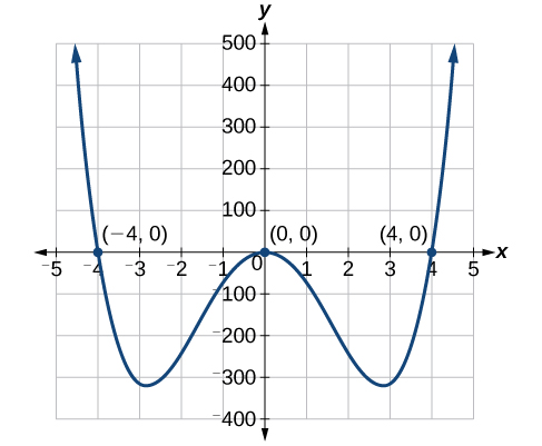
Figure 1
Example 5: Solve a Polynomial by Grouping
Solve a polynomial by grouping: [latex]{x}^{3}+{x}^{2}-9x - 9=0[/latex].
Solution
This polynomial consists of 4 terms, which we can solve by grouping. Grouping procedures require factoring the first two terms and then factoring the last two terms. If the factors in the parentheses are identical, we can continue the process and solve, unless more factoring is suggested.
The grouping process ends here, as we can factor [latex]{x}^{2}-9[/latex] using the difference of squares formula.
The solutions are [latex]x=3[/latex], [latex]x=-3[/latex], and [latex]x=-1[/latex]. Note that the highest exponent is 3 and we obtained 3 solutions. We can see the solutions, the x-intercepts, on the graph in Figure 2.
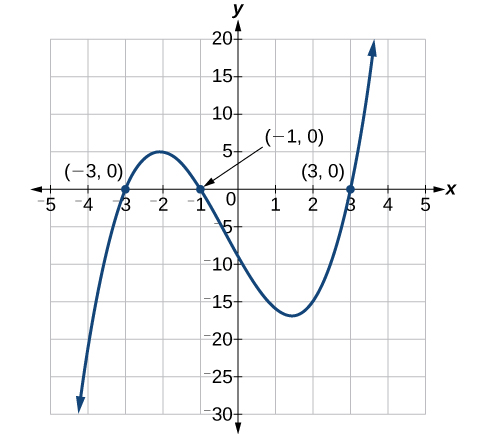
Figure 2
Analysis of the Solution
We looked at solving quadratic equations by factoring when the leading coefficient is 1. When the leading coefficient is not 1, we solved by grouping. Grouping requires four terms, which we obtained by splitting the linear term of quadratic equations. We can also use grouping for some polynomials of degree higher than 2, as we saw here, since there were already four terms.
Candela Citations
- College Algebra. Authored by: OpenStax College Algebra. Provided by: OpenStax. Located at: http://cnx.org/contents/9b08c294-057f-4201-9f48-5d6ad992740d@3.278:1/Preface. License: CC BY: Attribution