As part of exploring how functions change, we can identify intervals over which the function is changing in specific ways. We say that a function is increasing on an interval if the function values increase as the input values increase within that interval. Similarly, a function is decreasing on an interval if the function values decrease as the input values increase over that interval. The average rate of change of an increasing function is positive, and the average rate of change of a decreasing function is negative. Figure 3 shows examples of increasing and decreasing intervals on a function.
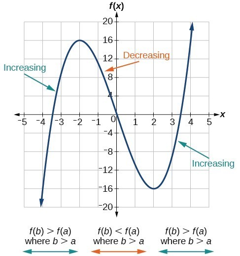
Figure 3. The function [latex]f\left(x\right)={x}^{3}-12x[/latex] is increasing on [latex]\left(-\infty \text{,}-\text{2}\right){{\cup }^{\text{ }}}^{\text{ }}\left(2,\infty \right)[/latex] and is decreasing on [latex]\left(-2\text{,}2\right)[/latex].
This video further explains how to find where a function is increasing or decreasing.
While some functions are increasing (or decreasing) over their entire domain, many others are not. A value of the input where a function changes from increasing to decreasing (as we go from left to right, that is, as the input variable increases) is called a local maximum. If a function has more than one, we say it has local maxima. Similarly, a value of the input where a function changes from decreasing to increasing as the input variable increases is called a local minimum. The plural form is “local minima.” Together, local maxima and minima are called local extrema, or local extreme values, of the function. (The singular form is “extremum.”) Often, the term local is replaced by the term relative. In this text, we will use the term local.
Clearly, a function is neither increasing nor decreasing on an interval where it is constant. A function is also neither increasing nor decreasing at extrema. Note that we have to speak of local extrema, because any given local extremum as defined here is not necessarily the highest maximum or lowest minimum in the function’s entire domain.
For the function in Figure 4, the local maximum is 16, and it occurs at [latex]x=-2[/latex]. The local minimum is [latex]-16[/latex] and it occurs at [latex]x=2[/latex].
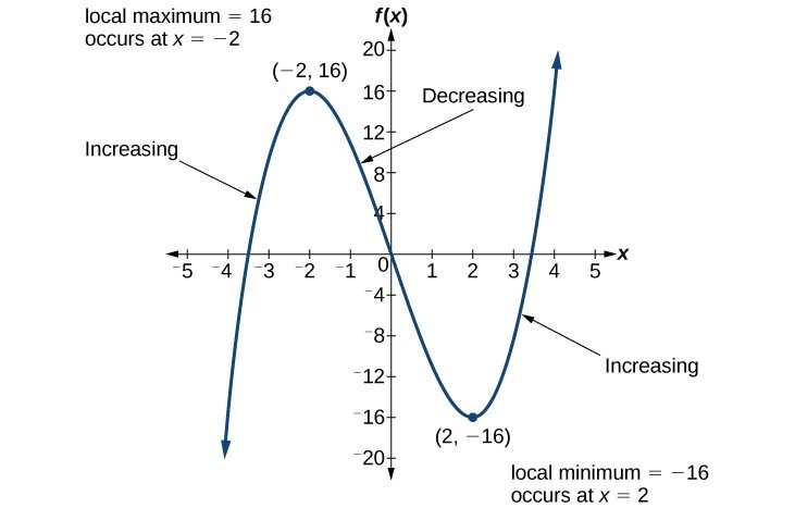
Figure 4
To locate the local maxima and minima from a graph, we need to observe the graph to determine where the graph attains its highest and lowest points, respectively, within an open interval. Like the summit of a roller coaster, the graph of a function is higher at a local maximum than at nearby points on both sides. The graph will also be lower at a local minimum than at neighboring points. Figure 5 illustrates these ideas for a local maximum.
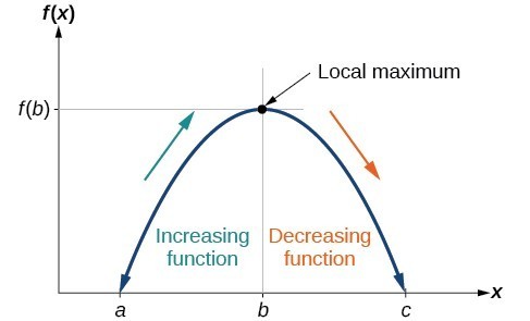
Figure 5. Definition of a local maximum.
These observations lead us to a formal definition of local extrema.
A General Note: Local Minima and Local Maxima
A function [latex]f[/latex] is an increasing function on an open interval if [latex]f\left(b\right)>f\left(a\right)[/latex] for any two input values [latex]a[/latex] and [latex]b[/latex] in the given interval where [latex]b>a[/latex].
A function [latex]f[/latex] is a decreasing function on an open interval if [latex]f\left(b\right)
A function [latex]f[/latex] has a local maximum at [latex]x=b[/latex] if there exists an interval [latex]\left(a,c\right)[/latex] with [latex]a
Example 7: Finding Increasing and Decreasing Intervals on a Graph
Given the function [latex]p\left(t\right)[/latex] in the graph below, identify the intervals on which the function appears to be increasing.
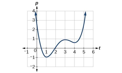
Figure 6
Solution
We see that the function is not constant on any interval. The function is increasing where it slants upward as we move to the right and decreasing where it slants downward as we move to the right. The function appears to be increasing from [latex]t=1[/latex] to [latex]t=3[/latex] and from [latex]t=4[/latex] on.
In interval notation, we would say the function appears to be increasing on the interval (1,3) and the interval [latex]\left(4,\infty \right)[/latex].
Example 8: Finding Local Extrema from a Graph
Graph the function [latex]f\left(x\right)=\frac{2}{x}+\frac{x}{3}[/latex]. Then use the graph to estimate the local extrema of the function and to determine the intervals on which the function is increasing.
Solution
Using technology, we find that the graph of the function looks like that in Figure 7. It appears there is a low point, or local minimum, between [latex]x=2[/latex] and [latex]x=3[/latex], and a mirror-image high point, or local maximum, somewhere between [latex]x=-3[/latex] and [latex]x=-2[/latex].
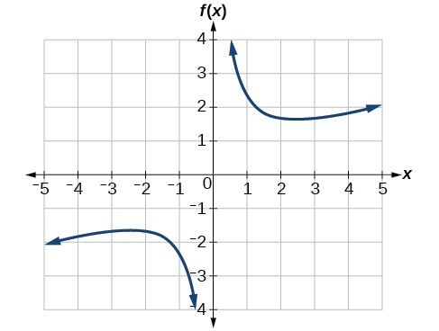
Figure 7
Analysis of the Solution
Most graphing calculators and graphing utilities can estimate the location of maxima and minima. Figure 7 provides screen images from two different technologies, showing the estimate for the local maximum and minimum.
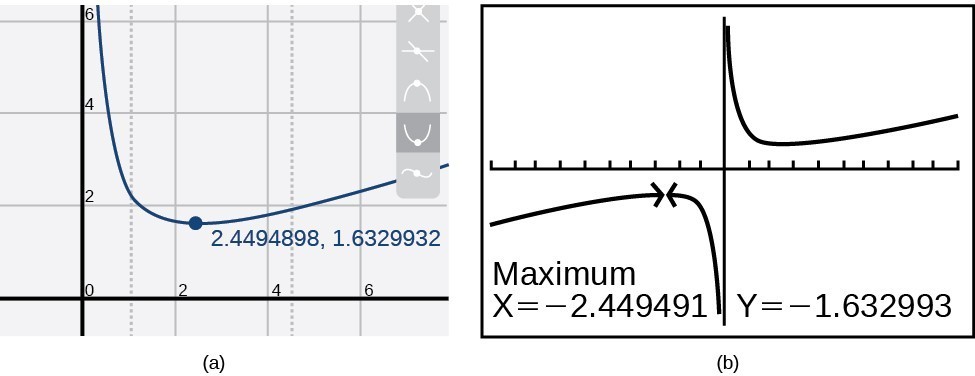
Figure 8
Based on these estimates, the function is increasing on the interval [latex]\left(-\infty ,-{2.449}\right)\\[/latex]
and [latex]\left(2.449\text{,}\infty \right)\\[/latex]. Notice that, while we expect the extrema to be symmetric, the two different technologies agree only up to four decimals due to the differing approximation algorithms used by each. (The exact location of the extrema is at [latex]\pm \sqrt{6}[/latex], but determining this requires calculus.)
Try It 4
Graph the function [latex]f\left(x\right)={x}^{3}-6{x}^{2}-15x+20\\[/latex] to estimate the local extrema of the function. Use these to determine the intervals on which the function is increasing and decreasing.
Example 9: Finding Local Maxima and Minima from a Graph
For the function [latex]f[/latex] whose graph is shown in Figure 9, find all local maxima and minima.
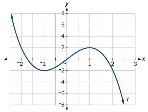
Figure 9
Solution
Observe the graph of [latex]f[/latex]. The graph attains a local maximum at [latex]x=1[/latex] because it is the highest point in an open interval around [latex]x=1[/latex]. The local maximum is the [latex]y[/latex] -coordinate at [latex]x=1[/latex], which is [latex]2[/latex].
The graph attains a local minimum at [latex]\text{ }x=-1\text{ }[/latex] because it is the lowest point in an open interval around [latex]x=-1[/latex]. The local minimum is the y-coordinate at [latex]x=-1[/latex], which is [latex]-2[/latex].
Analyzing the Toolkit Functions for Increasing or Decreasing Intervals
We will now return to our toolkit functions and discuss their graphical behavior in the table below.
| Function | Increasing/Decreasing | Example |
|---|---|---|
|
Constant Function [latex]f\left(x\right)={c}[/latex] |
Neither increasing nor decreasing |  |
|
Identity Function [latex]f\left(x\right)={x}[/latex] |
Increasing |  |
|
Quadratic Function [latex]f\left(x\right)={x}^{2}[/latex] |
Increasing on [latex]\left(0,\infty\right)[/latex] Decreasing on [latex]\left(-\infty,0\right)[/latex] Minimum at [latex]x=0[/latex] |
 |
|
Cubic Function [latex]f\left(x\right)={x}^{3}[/latex] |
Increasing |  |
|
Reciprocal [latex]f\left(x\right)=\frac{1}{x}[/latex] |
Decreasing [latex]\left(-\infty,0\right)\cup\left(0,\infty\right)[/latex] |  |
|
Reciprocal Squared [latex]f\left(x\right)=\frac{1}{{x}^{2}}[/latex] |
Increasing on [latex]\left(-\infty,0\right)[/latex] Decreasing on [latex]\left(0,\infty\right)[/latex] |
 |
|
Cube Root [latex]f\left(x\right)=\sqrt[3]{x}[/latex]
|
Increasing |  |
|
Square Root [latex]f\left(x\right)=\sqrt{x}[/latex] |
Increasing on [latex]\left(0,\infty\right)[/latex] |  |
|
Absolute Value [latex]f\left(x\right)=|x|[/latex] |
Increasing on [latex]\left(0,\infty\right)[/latex] Decreasing on [latex]\left(-\infty,0\right)[/latex] |
 |
Candela Citations
- Precalculus. Authored by: Jay Abramson, et al.. Provided by: OpenStax. Located at: http://cnx.org/contents/fd53eae1-fa23-47c7-bb1b-972349835c3c@5.175. License: CC BY: Attribution. License Terms: Download For Free at : http://cnx.org/contents/fd53eae1-fa23-47c7-bb1b-972349835c3c@5.175.
- Determine Where a Function is Increasing and Decreasing . Authored by: Mathispower4u. Located at: https://www.youtube.com/watch?v=78b4HOMVcKM. License: All Rights Reserved. License Terms: Standard YouTube License
Analysis of the Solution
Notice in this example that we used open intervals (intervals that do not include the endpoints), because the function is neither increasing nor decreasing at [latex]t=1[/latex] , [latex]t=3[/latex] , and [latex]t=4[/latex] . These points are the local extrema (two minima and a maximum).