Graphs behave differently at various x-intercepts. Sometimes, the graph will cross over the horizontal axis at an intercept. Other times, the graph will touch the horizontal axis and bounce off.
Suppose, for example, we graph the function
Notice in Figure 7 that the behavior of the function at each of the x-intercepts is different.
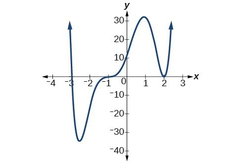
Figure 7. Identifying the behavior of the graph at an x-intercept by examining the multiplicity of the zero.
The x-intercept [latex]x=-3[/latex] is the solution of equation [latex]\left(x+3\right)=0[/latex]. The graph passes directly through the x-intercept at [latex]x=-3[/latex]. The factor is linear (has a degree of 1), so the behavior near the intercept is like that of a line—it passes directly through the intercept. We call this a single zero because the zero corresponds to a single factor of the function.
The x-intercept [latex]x=2[/latex] is the repeated solution of equation [latex]{\left(x - 2\right)}^{2}=0[/latex]. The graph touches the axis at the intercept and changes direction. The factor is quadratic (degree 2), so the behavior near the intercept is like that of a quadratic—it bounces off of the horizontal axis at the intercept.
The factor is repeated, that is, the factor [latex]\left(x - 2\right)[/latex] appears twice. The number of times a given factor appears in the factored form of the equation of a polynomial is called the multiplicity. The zero associated with this factor, [latex]x=2[/latex], has multiplicity 2 because the factor [latex]\left(x - 2\right)[/latex] occurs twice.
The x-intercept [latex]x=-1[/latex] is the repeated solution of factor [latex]{\left(x+1\right)}^{3}=0[/latex]. The graph passes through the axis at the intercept, but flattens out a bit first. This factor is cubic (degree 3), so the behavior near the intercept is like that of a cubic—with the same S-shape near the intercept as the toolkit function [latex]f\left(x\right)={x}^{3}[/latex]. We call this a triple zero, or a zero with multiplicity 3.
For zeros with even multiplicities, the graphs touch or are tangent to the x-axis. For zeros with odd multiplicities, the graphs cross or intersect the x-axis. See Figure 8 for examples of graphs of polynomial functions with multiplicity 1, 2, and 3.
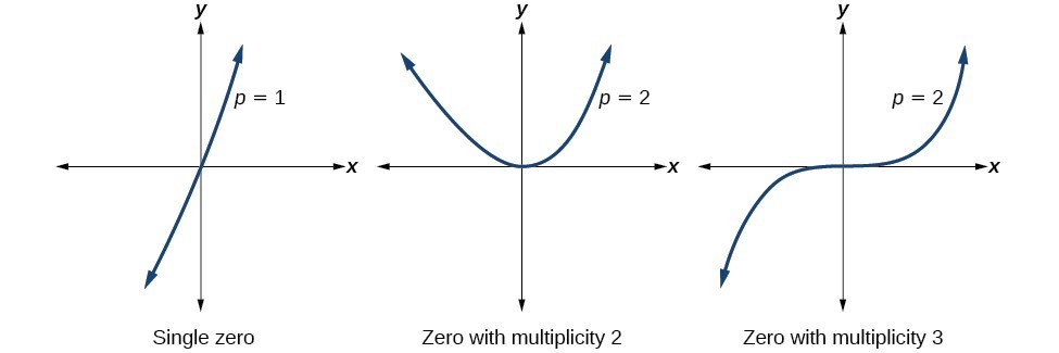
Figure 8
For higher even powers, such as 4, 6, and 8, the graph will still touch and bounce off of the horizontal axis but, for each increasing even power, the graph will appear flatter as it approaches and leaves the x-axis.
For higher odd powers, such as 5, 7, and 9, the graph will still cross through the horizontal axis, but for each increasing odd power, the graph will appear flatter as it approaches and leaves the x-axis.
A General Note: Graphical Behavior of Polynomials at x-Intercepts
If a polynomial contains a factor of the form [latex]{\left(x-h\right)}^{p}[/latex], the behavior near the x-intercept h is determined by the power p. We say that [latex]x=h[/latex] is a zero of multiplicity p.
The graph of a polynomial function will touch the x-axis at zeros with even multiplicities. The graph will cross the x-axis at zeros with odd multiplicities.
The sum of the multiplicities is the degree of the polynomial function.
How To: Given a graph of a polynomial function of degree n, identify the zeros and their multiplicities.
- If the graph crosses the x-axis and appears almost linear at the intercept, it is a single zero.
- If the graph touches the x-axis and bounces off of the axis, it is a zero with even multiplicity.
- If the graph crosses the x-axis at a zero, it is a zero with odd multiplicity.
- The sum of the multiplicities is n.
Example 6: Identifying Zeros and Their Multiplicities
Use the graph of the function of degree 6 to identify the zeros of the function and their possible multiplicities.
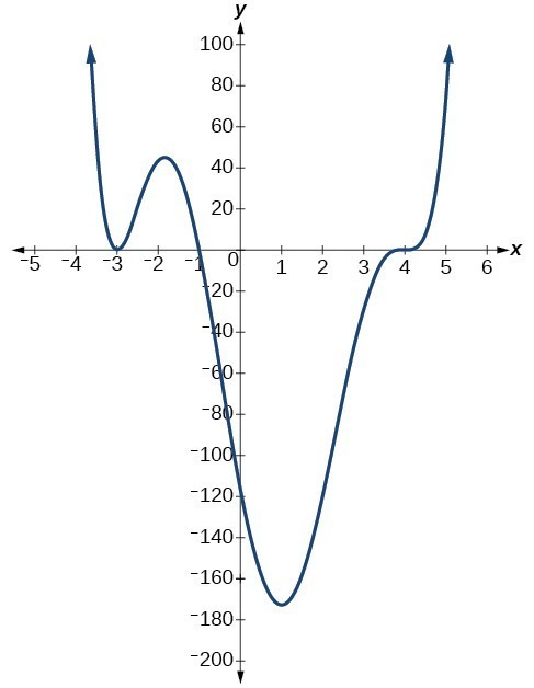
Figure 9
Solution
The polynomial function is of degree n. The sum of the multiplicities must be n.
Starting from the left, the first zero occurs at [latex]x=-3[/latex]. The graph touches the x-axis, so the multiplicity of the zero must be even. The zero of –3 has multiplicity 2.
The next zero occurs at [latex]x=-1[/latex]. The graph looks almost linear at this point. This is a single zero of multiplicity 1.
The last zero occurs at [latex]x=4[/latex]. The graph crosses the x-axis, so the multiplicity of the zero must be odd. We know that the multiplicity is likely 3 and that the sum of the multiplicities is likely 6.
Try It 2
Use the graph of the function of degree 5 to identify the zeros of the function and their multiplicities.
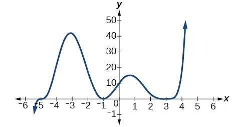
Figure 10
Determine end behavior
As we have already learned, the behavior of a graph of a polynomial function of the form
will either ultimately rise or fall as x increases without bound and will either rise or fall as x decreases without bound. This is because for very large inputs, say 100 or 1,000, the leading term dominates the size of the output. The same is true for very small inputs, say –100 or –1,000.
Recall that we call this behavior the end behavior of a function. As we pointed out when discussing quadratic equations, when the leading term of a polynomial function, [latex]{a}_{n}{x}^{n}[/latex], is an even power function, as x increases or decreases without bound, [latex]f\left(x\right)[/latex] increases without bound. When the leading term is an odd power function, as x decreases without bound, [latex]f\left(x\right)[/latex] also decreases without bound; as x increases without bound, [latex]f\left(x\right)[/latex] also increases without bound. If the leading term is negative, it will change the direction of the end behavior. The table below summarizes all four cases.
| Even Degree | Odd Degree |
|---|---|
 |
 |
 |
 |
Understand the relationship between degree and turning points
In addition to the end behavior, recall that we can analyze a polynomial function’s local behavior. It may have a turning point where the graph changes from increasing to decreasing (rising to falling) or decreasing to increasing (falling to rising). Look at the graph of the polynomial function [latex]f\left(x\right)={x}^{4}-{x}^{3}-4{x}^{2}+4x[/latex] in Figure 11. The graph has three turning points.
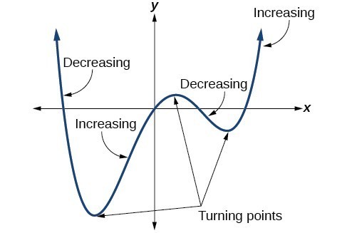
Figure 11
This function f is a 4th degree polynomial function and has 3 turning points. The maximum number of turning points of a polynomial function is always one less than the degree of the function.
A General Note: Interpreting Turning Points
A turning point is a point of the graph where the graph changes from increasing to decreasing (rising to falling) or decreasing to increasing (falling to rising).
A polynomial of degree n will have at most n – 1 turning points.
Example 7: Finding the Maximum Number of Turning Points Using the Degree of a Polynomial Function
Find the maximum number of turning points of each polynomial function.
- [latex]f\left(x\right)=-{x}^{3}+4{x}^{5}-3{x}^{2}++1[/latex]
- [latex]f\left(x\right)=-{\left(x - 1\right)}^{2}\left(1+2{x}^{2}\right)[/latex]
Solution
- [latex]f\left(x\right)=-x{}^{3}+4{x}^{5}-3{x}^{2}++1[/latex]
First, rewrite the polynomial function in descending order: [latex]f\left(x\right)=4{x}^{5}-{x}^{3}-3{x}^{2}++1[/latex]
Identify the degree of the polynomial function. This polynomial function is of degree 5.
The maximum number of turning points is 5 – 1 = 4.
- [latex]f\left(x\right)=-{\left(x - 1\right)}^{2}\left(1+2{x}^{2}\right)[/latex]

Figure 12
First, identify the leading term of the polynomial function if the function were expanded.
Then, identify the degree of the polynomial function. This polynomial function is of degree 4.
The maximum number of turning points is 4 – 1 = 3.
Candela Citations
- Precalculus. Authored by: Jay Abramson, et al.. Provided by: OpenStax. Located at: http://cnx.org/contents/fd53eae1-fa23-47c7-bb1b-972349835c3c@5.175. License: CC BY: Attribution. License Terms: Download For Free at : http://cnx.org/contents/fd53eae1-fa23-47c7-bb1b-972349835c3c@5.175.