Learning Objectives
- Represent a linear function in words, tabular form, with function notation, and with a graph
- Determine whether a linear function is increasing, decreasing, or constant
Just as with the growth of a bamboo plant, there are many situations that involve constant change over time. Consider, for example, the first commercial maglev train in the world, the Shanghai MagLev Train. It carries passengers comfortably for a 30-kilometer trip from the airport to the subway station in only eight minutes.[1]
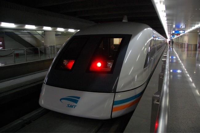
Suppose a maglev train were to travel a long distance, and that the train maintains a constant speed of 83 meters per second for a period of time once it is 250 meters from the station. How can we analyze the train’s distance from the station as a function of time? In this section, we will investigate a kind of function that is useful for this purpose, and use it to investigate real-world situations such as the train’s distance from the station at a given point in time.
The function describing the train’s motion is a linear function, which is defined as a function with a constant rate of change, that is, a polynomial of degree 1. There are several ways to represent a linear function, including word form, function notation, tabular form, and graphical form. We will describe the train’s motion as a function using each method.
Representing a Linear Function in Word Form
Let’s begin by describing the linear function in words. For the train problem we just considered, the following word sentence may be used to describe the function relationship.
- The train’s distance from the station is a function of the time during which the train moves at a constant speed plus its original distance from the station when it began moving at constant speed.
The speed is the rate of change. Recall that a rate of change is a measure of how quickly the dependent variable changes with respect to the independent variable. The rate of change for this example is constant, which means that it is the same for each input value. As the time (input) increases by 1 second, the corresponding distance (output) increases by 83 meters. The train began moving at this constant speed at a distance of 250 meters from the station.
Representing a Linear Function in Function Notation
Another approach to representing linear functions is by using function notation. One example of function notation is an equation written in the form known as the slope-intercept form of a line, where [latex]x[/latex] is the input value, [latex]m[/latex] is the rate of change, and [latex]b[/latex] is the initial value of the dependent variable.
[latex]\begin{array}{l}\text{Equation form}\hfill & y=mx+b\hfill \\ \text{Equation notation}\hfill & f\left(x\right)=mx+b\hfill \end{array}[/latex]
In the example of the train, we might use the notation [latex]D\left(t\right)[/latex] in which the total distance [latex]D[/latex] is a function of the time [latex]t[/latex]. The rate, [latex]m[/latex], is 83 meters per second. The initial value of the dependent variable [latex]b[/latex] is the original distance from the station, 250 meters. We can write a generalized equation to represent the motion of the train.
[latex]D\left(t\right)=83t+250[/latex]
Representing a Linear Function in Tabular Form
A third method of representing a linear function is through the use of a table. The relationship between the distance from the station and the time is represented in the table below. From the table, we can see that the distance changes by 83 meters for every 1 second increase in time.
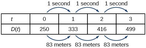
Tabular representation of the function D showing selected input and output values
Q & A
Can the input in the previous example be any real number?
No. The input represents time, so while nonnegative rational and irrational numbers are possible, negative real numbers are not possible for this example. The input consists of non-negative real numbers.
Try It
Representing a Linear Function in Graphical Form
Another way to represent linear functions is visually, using a graph. We can use the function relationship from above, [latex]D\left(t\right)=83t+250[/latex], to draw a graph, represented in the graph below. Notice the graph is a line. When we plot a linear function, the graph is always a line.
The rate of change, which is constant, determines the slant, or slope of the line. The point at which the input value is zero is the vertical intercept, or y-intercept, of the line. We can see from the graph that the y-intercept in the train example we just saw is [latex]\left(0,250\right)[/latex] and represents the distance of the train from the station when it began moving at a constant speed.
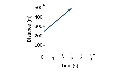
The graph of [latex]D\left(t\right)=83t+250[/latex]. Graphs of linear functions are lines because the rate of change is constant.
Notice that the graph of the train example is restricted, but this is not always the case. Consider the graph of the line [latex]f\left(x\right)=2{x}_{}+1[/latex]. Ask yourself what numbers can be input to the function, that is, what is the domain of the function? The domain is comprised of all real numbers because any number may be doubled, and then have one added to the product.
A General Note: Linear Function
A linear function is a function whose graph is a line. Linear functions can be written in the slope-intercept form of a line
[latex]f\left(x\right)=mx+b[/latex]
where [latex]b[/latex] is the initial or starting value of the function (when input, [latex]x=0[/latex]), and [latex]m[/latex] is the constant rate of change, or slope of the function. The y-intercept is at [latex]\left(0,b\right)[/latex].
Try It
Example: Using a Linear Function to Find the Pressure on a Diver
The pressure, [latex]P[/latex], in pounds per square inch (PSI) on the diver in Figure 3 depends upon her depth below the water surface, [latex]d[/latex], in feet. This relationship may be modeled by the equation, [latex]P\left(d\right)=0.434d+14.696[/latex]. Restate this function in words.

(credit: Ilse Reijs and Jan-Noud Hutten)
Try it now
Use Desmos to graph the function: [latex]f(x)=-\frac{2}{3}x-\frac{4}{3}[/latex].
![]()
Now watch this short tutorial on how to add sliders to your graphs.
Now add a slider to the function [latex]f(x) =-\frac{2}{3}x-\frac{4}{3}[/latex] that will let you change the slope. Limit the range of values for the slope such that your function is increasing, then do the same for a function that is decreasing. Finally, write and graph a function whose slope is constant.
Determine Whether a Linear Function is Increasing, Decreasing, or Constant
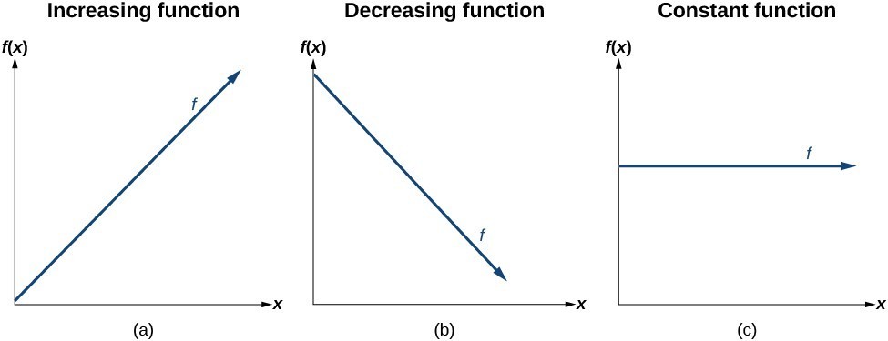
The linear functions we used in the two previous examples increased over time, but not every linear function does. A linear function may be increasing, decreasing, or constant. For an increasing function, as with the train example, the output values increase as the input values increase. The graph of an increasing function has a positive slope. A line with a positive slope slants upward from left to right as in (a). For a decreasing function, the slope is negative. The output values decrease as the input values increase. A line with a negative slope slants downward from left to right as in (b). If the function is constant, the output values are the same for all input values so the slope is zero. A line with a slope of zero is horizontal as in (c).
A General Note: Increasing and Decreasing Functions
The slope determines if the function is an increasing linear function, a decreasing linear function, or a constant function.
- [latex]f\left(x\right)=mx+b\text{ is an increasing function if }m>0[/latex].
- [latex]f\left(x\right)=mx+b\text{ is an decreasing function if }m<0[/latex].
- [latex]f\left(x\right)=mx+b\text{ is a constant function if }m=0[/latex].
Example: Deciding whether a Function Is Increasing, Decreasing, or Constant
Some recent studies suggest that a teenager sends an average of 60 texts per day.[2] For each of the following scenarios, find the linear function that describes the relationship between the input value and the output value. Then, determine whether the graph of the function is increasing, decreasing, or constant.
- The total number of texts a teen sends is considered a function of time in days. The input is the number of days, and output is the total number of texts sent.
- A teen has a limit of 500 texts per month in his or her data plan. The input is the number of days, and output is the total number of texts remaining for the month.
- A teen has an unlimited number of texts in his or her data plan for a cost of $50 per month. The input is the number of days, and output is the total cost of texting each month.
Candela Citations
- Revision and Adaptation. Provided by: Lumen Learning. License: CC BY: Attribution
- Question ID 113465. Authored by: Lumen Learning. License: CC BY: Attribution. License Terms: IMathAS Community License CC-BY + GPL
- College Algebra. Authored by: Abramson, Jay et al.. Provided by: OpenStax. Located at: http://cnx.org/contents/9b08c294-057f-4201-9f48-5d6ad992740d@5.2. License: CC BY: Attribution. License Terms: Download for free at http://cnx.org/contents/9b08c294-057f-4201-9f48-5d6ad992740d@5.2
- Question ID 2923. Authored by: Anderson,Tophe. License: CC BY: Attribution. License Terms: IMathAS Community License CC-BY + GPL