Learning Objectives
- Use probability distributions for discrete and continuous random variables to estimate probabilities and identify unusual events.
The Mean and Standard Deviation of a Discrete Random Variable
We now focus on the mean and standard deviation of a discrete random variable. We discuss how to calculate these measures of center and spread for this type of probability distribution, but in general we will use technology to do these calculations.
Example
The Mean of a Discrete Random Variable
At Rushmore Community College, there have been complaints about how long it takes to get food from the college cafeteria. In response, a study was conducted to record the total amount of time students had to wait to get their food. The following table gives the total times (rounded to the nearest 5 minutes) to get food for 200 randomly selected students.
Here is the frequency table.
| Time (minutes) | 5 | 10 | 15 | 20 | 25 |
| Number of students | 30 | 52 | 62 | 40 | 16 |
Using this data, we can create a probability distribution for the random variable X = “time to get food.” As we have done before, we divide each frequency (count) by the total number of observations. For example, to calculate the probability that a student will have to wait 10 minutes to get their food we divide: (the number of students in the sample that waited 10 minutes) by (the total number of students in the sample) = 52 / 200 = 0.26.
| X = Time (minutes) | 5 | 10 | 15 | 20 | 25 |
| P(X) | 30 / 200 = 0.15 | 52 / 200 = 0.26 | 62 / 200 = 0.31 | 40 / 200 = 0.20 | 16 / 200 = 0.08 |
Here is the corresponding probability histogram:

A comment on probability histograms
In this probability histogram, the area, instead of the height, is the probability. In general, when we work with probability histograms, the area will represent the probability, so we will not worry about the units on the y-axis. Since the area represents the probabilities, the total area is 1.
Because in this case we have the actual data in the first table, we start by using that table of actual counts to calculate the mean. However, usually all we have is the probability distribution, so we will also consider how to calculate the mean directly from this information alone.
Calculating the Mean from the Frequency Table
| Time (minutes) | 5 | 10 | 15 | 20 | 25 |
| Number of students | 30 | 52 | 62 | 40 | 16 |
We have 200 observations that are summarized in this table. We have 30 students with a time of 5 minutes, 52 students with a time of 10 minutes, 62 students with a time of 15 minutes, and so on.
To calculate the mean (that is the average), we have to add 30 fives + 52 tens + 62 fifteens + 40 twenties + 16 twenty-fives and then divide by 200. Here is that calculation:
[latex]\frac{\text{5}(\text{30})+\text{10}(\text{52})+\text{15}(\text{62})+\text{20}(\text{40})+\text{25}(\text{16})}{\text{200}}=\text{14}[/latex]
So the mean time for students to get their food in the cafeteria is 14 minutes.
Calculating the Mean from the Probability Distribution
Now let’s take a closer look at the calculation we just did.
Notice that the large fraction on the left could be broken up into a sum of five smaller fractions all with the denominator 200:
[latex]\frac{\text{5}(\text{30})}{\text{200}}+\frac{\text{10}(\text{52})}{\text{200}}+\frac{\text{15}(\text{62})}{\text{200}}+\frac{\text{20}(\text{40})}{\text{200}}+\frac{\text{25}(\text{16})}{\text{200}}=\text{14}[/latex]
Okay, we are almost there. The last thing to do is rewrite each of these fractions like this:
[latex]\text{5}\left(\frac{30}{200}\right)+\text{10}\left(\frac{52}{200}\right)+\text{15}\left(\frac{62}{200}\right)+\text{20}\left(\frac{40}{200}\right)+\text{25}\left(\frac{16}{200}\right)=\text{14}[/latex]
Here is the same equation with the fractions expressed as decimals:
[latex]\text{5}\left(0.15\right)+\text{10}\left(0.26\right)+\text{15}\left(0.31\right)+\text{20}\left(0.20\right)+\text{25}\left(0.08\right)=\text{14}[/latex]
Look closely at the terms we are adding. In each case, we have the product of one of the possible values of X and its corresponding probability:
| X = Time (minutes) | 5 | 10 | 15 | 20 | 25 |
| P(X) | 30 / 200 = 0.15 | 52 / 200 = 0.26 | 62 / 200 = 0.31 | 40 / 200 = 0.20 | 16 / 200 = 0.08 |
As we can see, the mean is just a weighted average. That is, the mean is the weighted sum of all the possible values of the random variable X, where each value is weighted by its probability.
Comment
Why Is the Mean a Weighted Average?
The mean of a discrete random variable X should give us a measure of the long-run average value for X. It therefore makes sense to count more heavily those values of X that have a high probability, because they are more likely to occur and will consequently influence the long-run average. On the other hand, those values of X with low probability will not occur very often, so they will have little effect on the long-run average. It therefore makes sense to not give them much weight in our calculation.
The Formula for the Mean of a Discrete Random Variable
Earlier in the course, when we calculated the mean of a data set, we used the symbol [latex]\stackrel{¯}{x}[/latex] (x-bar) to represent that value. We do not use [latex]\stackrel{¯}{x}[/latex] to represent the mean of a random variable; instead we use [latex]{\mathrm{μ}}_{x}[/latex] (pronounced “mu-sub-x”).
Here is the formula that we have come up with for the mean of a discrete random variable. Note that [latex]P(x)[/latex] represents the probability of x, where x is a value of the random variable X.

Another term often used to describe the mean is expected value. It is a useful term because it reminds us that the mean of a random variable is not calculated on a fixed data set. Rather, the mean (expected value) is a measure of the expected long-term behavior of the random variable.
Learn By Doing
Drivers entering the short-term parking facility at an airport are given the option to purchase a parking permit for one of four possible time periods: ½ hour, 1 hour, 1½ hours, or 2 hours. Thus, for each driver who enters the parking facility, we can consider their choice of parking time as a discrete random variable. In this case, the random variable X has four possible values: 0.5, 1, 1.5, and 2.
Assume that the probability distribution for X is given by the following table.
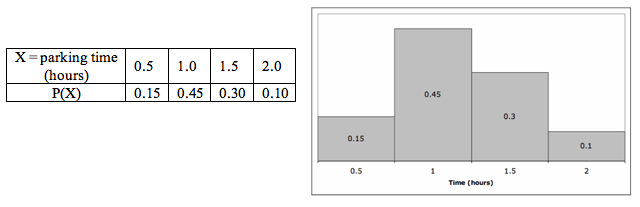
For example, reading from this table, it appears that there is a 15% chance that the next driver entering the parking facility will opt for a ½-hour permit. In the probability histogram, the area of each rectangle (not the height) is the probability of the corresponding x-value occurring.
Candela Citations
- Concepts in Statistics. Provided by: Open Learning Initiative. Located at: http://oli.cmu.edu. License: CC BY: Attribution