Learning Objectives
- Use probability distributions for discrete and continuous random variables to estimate probabilities and identify unusual events.
Here is another example of how to use the mean and standard deviation of a discrete random variable to identify unusual values for a random variable.
Example
Changing Majors
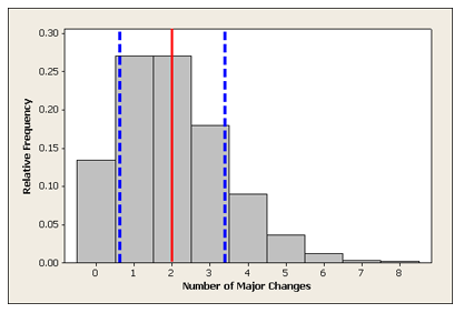
Here we have again the probability distribution of the number of changes in major.
| X | 0 | 1 | 2 | 3 | 4 | 5 | 6 | 7 | 8 |
| P(X) | 0.135 | 0.271 | 0.271 | 0.180 | 0.090 | 0.036 | 0.012 | 0.003 | 0.002 |
How often do we expect a college student to change majors?
This question is asking for the expected value, which is the mean of the probability distribution. So we calculate the weighted average, as before:
[latex]0(0.135)+1(0.271)+2(0.271)+3(0.180)+4(0.090)+5(0.036)+6(0.012)+7(0.003)+8(0.002)=2[/latex]
What is the standard deviation of the probability distribution?
[latex]\sqrt{{(0-2)}^{2}(0.135)+{(1-2)}^{2}(0.271)+{(2-2)}^{2}(0.271)+{(3-2)}^{2}(0.180)+{(4-2)}^{2}(0.090)+...+{(7-2)}^{2}(0.003)+{(8-2)}^{2}(0.002)}\approx 1.4[/latex]
We have drawn lines to show the mean and 1 standard deviation above and below the mean.
Recall that earlier, we discussed what would be considered an unusual (and not unusual) number of changes in major, and we used probability calculations to assess that. For example, we found that changing majors 5 or more times occurs only about 5% of the time and therefore can be considered unusual.
Another way to think about defining “unusual” is to look at outcomes relative to the mean. We might consider outcomes more than 2 standard deviations above the mean as unusual.
What values are more than 2 standard deviations above the mean of 2?
Mean + 2 (standard deviation) = [latex]{\mathrm{μ}}_{x}+2⋅\mathrm{SD}=2+2⋅1.4=4.8[/latex], which rounds to 5.
We conclude from this line of reasoning that a college student who changes majors 5 or more times is “unusual.”
In Summarizing Data Graphically and Numerically, we used the standard deviation to identify usual, or typical, values. We said that a typical range of values falls within 1 standard deviation of the mean. We can use a similar idea here.
Learn By Doing
Example
Detecting Fraud
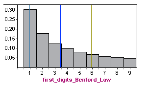
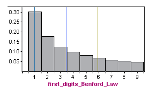
Legitimate records often display a surprising pattern that is not present in faked tax returns or other fraudulent accounting records. In legitimate records, the distribution of first digits can be modeled using Benford’s law. For example, suppose the total income recorded on a tax return is $20,712. The first digit is 2. Now we examine a very large number of tax returns and record the first digit of total income for all of the returns. The relative frequency of each first digit will behave according to Benford’s law.

Benford’s law can also be described using a mathematical formula, but we will not go into that here. Instead, let’s double-check that this distribution meets the criteria for a probability distribution of a discrete random variable. For a randomly selected tax return, we cannot predict what the first digit will be, but the first digits behave according to a predictable pattern described by Benford’s law. The model assigns probabilities to all possible values for a first digit (notice that the first digit cannot be zero). All possible outcomes taken together have a probability of 1. You can verify this by adding together the probabilities in the table.
Here is the probability distribution for first digits based on Benford’s law shown in a histogram. The mean is approximately 3.4, with a standard deviation of about 2.5 (calculations not shown).
Now, let’s compare this distribution to real data.
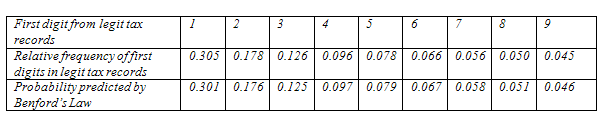
The second line in the following table is the probability distribution for the first significant digit in true tax data collected by Mark Nigrini from 169,662 IRS model files. You can see that relative frequencies of first digits in the legitimate tax records follow Benford’s law very closely.
By comparison, here is the probability distribution for first digits in fraudulent tax records from a study of fraudulent cash disbursement and payroll expenditures conducted in 1995 by the district attorney’s office in Kings County, New York. For fraudulent data, the mean is approximately 5.2, with a standard deviation of about 0.9.
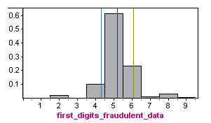
Obviously, the relative frequencies of first digits from the fraudulent data do not follow Benford’s law (shown again below). The distributions have very different shapes, means, and standard deviations. Compared to legitimate data, in fraudulent data, we are much more likely to see numbers with a first digit of 5 and much less likely to see numbers with a first digit of 1, 2, or 3.
Comment
When we compare the two distributions above, we can get a better understanding of the standard deviation of a random variable. The distribution in which it is more likely to find values that are further from the mean will have a larger standard deviation.
Likewise, the distribution in which it is less likely to find values that are further from the mean will have a smaller standard deviation.
In the fraudulent distribution, values like 1 or 2 that are far from the mean are very unlikely. On the other hand, in the Benford’s law distribution, the values 1 and 2 are quite likely. Indeed, the standard deviation of the Benford law is 2.5, which is larger than the standard deviation of 0.9 in the fraudulent distribution.
Learn By Doing
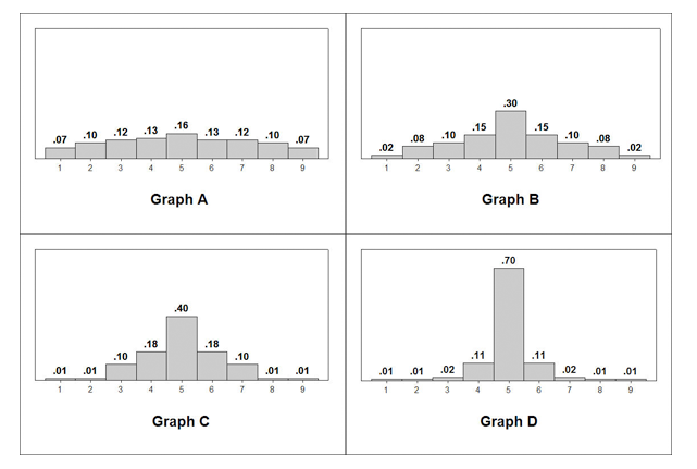
Use the following histograms to answer the activity question:
 https://assessments.lumenlearning.com/assessments/3563
Let’s Summarize
- The probability of an event is a measure of the likelihood that the event occurs.
- Probabilities are always between 0 and 1. The closer the probability is to 0, the less likely the event is to occur. The closer the probability is to 1, the more likely the event is to occur.
- The two ways of determining probabilities are empirical and theoretical.
- Empirical methods use a series of trials that produce outcomes that cannot be predicted in advance (hence the uncertainty). The probability of an event is approximated by the relative frequency of the event.
- Theoretical methods use the nature of the situation to determine probabilities. Probability rules allow us to calculate theoretical probabilities.
- Some common probability rules:
- The probability of the complement of an event A can be found by subtracting the probability of A from 1: P(not A) = 1 – P(A)
- Events are called disjoint or mutually exclusive if they have no events in common. If A and B are disjoint events, then P(A or B) = P(A) + P(B).
- When the knowledge of the occurrence of one event A does not affect the probability of another event B, we say the events are independent. If A and B are independent events, then P(A and B) = P(A) · P(B).
- When we have a quantitative variable with outcomes that occur as a result of some random process (e.g., rolling a die, choosing a person at random), we call it a random variable.
- There are two types of random variables:
- Discrete random variables have numeric values that can be listed and often can be counted.
- Continuous random variables can take any value in an interval and are often measurements. This type of random variable will be discussed in section 6.2.
- A probability distribution of a random variable tells us the probabilities of all the possible outcomes (for discrete random variables) of the variable or ranges of values (for continuous random variables). A probability distribution shows us the regular, predictable distribution of outcomes in a large number of repetitions of a random variable.
- For a discrete random variable, the probabilities of values are areas of the corresponding regions of the probability histogram for the variable.
Candela Citations
- Concepts in Statistics. Provided by: Open Learning Initiative. Located at: http://oli.cmu.edu. License: CC BY: Attribution