Learning Objectives
- Conduct a hypothesis test for a population proportion. State a conclusion in context.
On the previous page, we looked at determining hypotheses for testing a claim about a population proportion. On this page, we look at how to determine P-values.
As we learned earlier, the P-value for a hypothesis test for a population proportion comes from a normal model for the sampling distribution of sample proportions. The normal distribution is an appropriate model for this sampling distribution if the expected number of success and failures are both at least 10. Using the symbols for the population proportion and sample size, a normal curve is a reasonable model if the following conditions are met: np ≥ 10 and n(1 − p) ≥ 10.
Example
Health Insurance Coverage
Recall this example from the previous page. According to the Government Accountability Office, 80% of all college students (ages 18 to 23) had health insurance in 2006. The Patient Protection and Affordable Care Act of 2010 allowed young people under age 26 to stay on their parents’ health insurance policy. Has the proportion of college students (ages 18 to 23) who have health insurance increased since 2006? A survey of 800 randomly selected college students (ages 18 to 23) indicated that 83% of them had health insurance. Use a 0.05 level of significance.
Step 1: Determine the hypotheses.
We did this on the previous page. The hypotheses are:
- H0: p = 0.80
- Ha: p > 0.80
where p is the proportion of college students ages 18 to 23 who have health insurance now.
Step 2: Collect the data.
In this random sample of 800 college students, 83% have health insurance. If 80% of all college students have health insurance, is this 3% difference statistically significant or due to chance? We need to find a P-value to answer this question. We must determine if we can use this data in a hypothesis test.
First note that the data are from a random sample. That is essential. Now we need to determine if a normal model is a good fit for the sampling distribution. Since we assume that the null hypothesis is true, we build the sampling distribution with the assumption that 0.80 is the population proportion. We check the following conditions, using 0.80 for p:
[latex]np=(800)(0.80)=640\text{ }\mathrm{and}\text{ }n(1-p)=(800)(1-0.80)=160[/latex]
Because these are both more than 10, we can use the normal model to find the P-value.
Step 3: Assess the evidence.
Now that we know that the normal distribution is an appropriate model for the sampling distribution, our next goal is to determine the P-value. The first step is to determine the z-score for the observed sample proportion (the data).
The sample proportion is 0.83. Recall from Linking Probability to Statistical Inference that the formula for the z-score of a sample proportion is as follows:
[latex]Z=\frac{\stackrel{ˆ}{p}-p}{\sqrt{\frac{p(1-p)}{n}}}[/latex]
For this example, we calculate:
[latex]Z=\frac{0.83-0.80}{\sqrt{\frac{0.80(1-0.80)}{800}}}\approx 2.12[/latex]
This z-score is called the test statistic. It tells us the sample proportion of 0.83 is about 2.12 standard errors above the population proportion given in the null hypothesis. We use this statistic to find the P-value. The P-value describes the strength of the evidence against the null hypothesis.
We use the simulation that we first saw in Probability and Probability Distributions to determine the P-value. The P-value is a probability that describes the likelihood of the data if the null hypothesis is true. More specifically, the P-value is the probability that sample results are as extreme as or more extreme than the data if the null hypothesis is true. The phrase “as extreme as or more extreme than” means farther from the center of the sampling distribution in the direction of the alternative hypothesis.
In this situation, we want the area to the right of 0.83 because the alternative hypothesis is a “greater-than” statement. The P-value, in this case, is the probability of getting a sample proportion equal to or greater than 0.83. Since we are using the standard normal curve to find probabilities, the P-value is the area to the right of the Z = 2.12.

We can find this area with a simulation or other technology.

The P-value is approximately 0.0170. Thus, the probability that a random sample proportion is at least as large as 0.83 is about 0.017 (if the population proportion is actually 0.80). If the null hypothesis is true, we observe sample proportions this high or higher only about 1.7% of the time.
The P-value is our evidence of statistical significance. It is a measure of whether random chance can explain the deviation of the data from the null hypothesis.
Step 4: State a conclusion.
To determine our conclusion, we compare the P-value to the level of significance, α = 0.05. If our data are predicted to occur by chance less than 5% of the time, we have reason to reject the null hypothesis and accept the alternative. Since our P-value of 0.017 is less than 0.05, we reject the null hypothesis. We state our conclusion in terms of the alternative hypothesis. We also state it in context.
The data from this study provides strong evidence that the proportion of all college students who have health insurance is now greater than 0.80 (P-value = 0.017). The 0.03 increase in the proportion who have health insurance since 2008 is statistically significant at the 0.05 level.
Alternatively, we can give the conclusion using the percentage rather than the decimal:
The data from this study provides strong evidence that the percentage of all college students who have health insurance is now greater than 80% (P-value = 0.017). The 3% increase in the percentage who have health insurance since 2008 is statistically significant at the 5% level.
Important Note
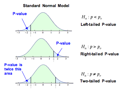
A hypothesis test can be one-tailed or two-tailed. The previous example was a one-tailed hypothesis test. The P-value was the area of the right tail. If the inequality in the alternative hypothesis is < or >, the test is one-tailed. If the inequality is ≠, the test is two-tailed.
Example
Internet Access
Recall the following example from the previous page. According to the Kaiser Family Foundation, 84% of U.S. children iages 8 to 18 had Internet access at home as of August 2009. Researchers wonder if this percentage has changed since then. They survey 500 randomly selected children (ages 8 to 18) and find that 430 of them have Internet access at home.
Use a level of significance of α = 0.05 for this hypothesis test.
Step 1: Determine the hypotheses.
- H0: p = 0.84
- Ha: p ≠ 0.84
where p is the proportion of children ages 8 to 18 with Internet access at home now.
Step 2: Collect the data.
Our sample is random, so there is no problem there. Again, we want to determine whether the normal model is a good fit for the sampling distribution of sample proportions. Based on the null hypothesis, we will use 0.84 as our population proportion to check the conditions.
[latex]np=(500)(0.84)=420\text{ }\mathrm{and}\text{ }n(1-p)=(500)(1-0.84)=80[/latex]
Because these are both more than 10, we can use the normal model to find the P-value.
Step 3: Assess the evidence.
Since we can use the normal model, we need to calculate the z-test statistic for the sample proportion. We first calculate the sample proportion.
[latex]\stackrel{ˆ}{p}=\frac{x}{n}=\frac{430}{500}=0.86[/latex]
Next, we calculate our Z-score, the test statistic:
[latex]Z=\frac{\stackrel{ˆ}{p}-p}{\sqrt{\frac{p(1-p)}{n}}}=\frac{0.86-0.84}{\sqrt{\frac{0.84(1-0.84)}{500}}}\approx 1.22[/latex]
The sample proportion of 0.86 is about 1.22 standard errors above the population proportion given in the null hypothesis. Now we calculate the P-value. This is where the two-tailed nature of the test is important. The P-value is the probability of seeing a sample proportion at least as extreme as the one observed from the data if the null hypothesis is true.
In the previous example, only sample proportions higher than the null proportion were evidence in favor of the alternative hypothesis. In this example, any sample proportion that differs from 0.84 is evidence in favor of the alternative. Statistically significant differences are at least as extreme as the difference we see in the data. We want to determine the probability that the difference in either direction (above or below 0.84) is at least as large as the difference seen in the data, so we include sample proportions at or above 0.86 and sample proportions at or below 0.82. For this reason, we look at the area in both tails. Our simulation shows one tail, so we have to double this area.
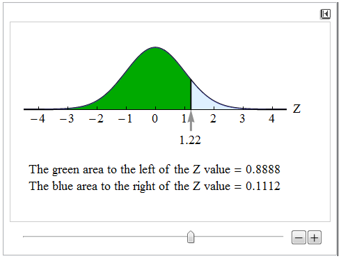
The area above the test statistic of 1.22 is about 0.11. We double this area to include the area in the left tail, below Z = −1.22. This gives us a P-value of approximately 0.22.
Our sample proportion was 0.02 above the population proportion from the null hypothesis. In a sample of size 500, we would observe a sample proportion 0.02 or more away from 0.84 about 22% of the time by chance alone.
Step 4: State a conclusion.
Again we compare the P-value to the level of significance, α = 0.05. In this case, the P-value of 0.22 is greater than 0.05, which means we do not have enough evidence to reject the null hypothesis. A sample result that could occur 22% of the time by chance alone is not statistically significant. Now we can state the conclusion in terms of the alternative hypothesis.
The data from this study does not provide evidence that is strong enough to conclude that the proportion of all children ages 8 to 18 who have Internet access at home has changed since 2009 (P-value = 0.22). The 2% change observed in the data is not statistically significant. These results can be explained by predictable variation in random samples.
A Note about the Conclusion
In the conclusion above, we did not have enough evidence to reject the null hypothesis. As we noted in “Hypothesis Testing,” failing to reject the null hypothesis does not mean the null hypothesis is true.
In the case of the previous example, it is possible that the proportion of children who have Internet access at home has changed. But the data we gathered did not provide the evidence to detect that the proportion had changed significantly.
Researchers often note improvements that could be made in their research and suggest follow-up research that might be done. In our example, a second sample with a larger sample size might provide the evidence needed to reject the null hypothesis.
The important thing to keep in mind is that at the end of a hypothesis test, we never say that the null hypothesis is true.
Learn By Doing
California College Students Who Drink
According to the Centers for Disease Control and Prevention, 60% of all American adults ages 18 to 24 currently drink alcohol. Is the proportion of California college students who currently drink alcohol different from the proportion nationwide? A survey of 450 California college students indicates that 66% currently drink alcohol. The hypotheses were:
- H0: p = 0.60
- Ha: p ≠ 0.60
Click here to open the simulation
Learn By Doing
Coin Flips
Recall the scenario from the previous page. A psychic claims to be able to predict the outcome of coin flips before they happen. Someone who guesses randomly will predict about half of coin flips correctly. In 100 flips, the psychic correctly predicts 57 flips. Do the results of this test indicate that the psychic does better than random guessing? The hypotheses are
- H0: p = 0.50
- Ha: p > 0.50
where p is the proportion of correct coin flip predictions by the psychic.
Click here to open the simulation
Learn By Doing
Candela Citations
- Concepts in Statistics. Provided by: Open Learning Initiative. Located at: http://oli.cmu.edu. License: CC BY: Attribution