Learning Objectives
- Use a five-number summary and a boxplot to describe a distribution.
Introduction
On the previous page, we learned about the five-number summary. At this point, you should know the following:
- The five-number summary uses quartiles to identify the center and spread of a distribution.
- The median (which is Q2) is a measure of center. We also view the median as a typical value that represents the distribution.
- The values between Q1 and Q3 give a typical range of values.
- The IQR is a way to measure the variability about the median.
Now we use the five-number summary to make a new type of graph, the boxplot. Boxplots are commonly used to summarize a distribution of a quantitative variable.
Example
Boxplots for Exam Scores
Here are the two sets of exam scores from the previous example. Recall that we divided the data into quartiles. In a data set, each quartile contains the same number of scores. In other words, each quartile contains 25% of the data.
Here is the five-number summary for these two distributions:
- Class A: Min: 40 Q1: 71 Q2: 74.5 Q3: 78.5 Max: 95
- Class B: Min: 40 Q1: 61 Q2: 74.5 Q3: 89 Max: 95
To create the boxplot for each distribution,
- Draw a box from Q1 to Q3.
- Draw a vertical line in the box at the median.
- Extend a tail from Q1 to the smallest value that is not an outlier and from Q3 to the largest value that is not an outlier.
- Indicate outliers with asterisks (*).

Notice: A long box in the boxplot indicates a large IQR, so the middle half of the data has a lot of variability. A short box in the boxplot indicates a small IQR. In this case, the middle half of the data has little variability.
Frequently, side-by-side boxplots are drawn vertically. Here we drew vertical dotplots with their boxplots for the exam scores from the two classes.

Note: Some statistical packages offer two options: a boxplot and a modified boxplot. We drew modified boxplots in this example. In a modified boxplot, outliers are marked with an asterisk (*). For a boxplot that is not modified, the tails extend to the minimum and maximum values. In this type of boxplot, we cannot see outliers.
Making a Boxplot:
Now we walk through the steps for making a modified boxplot using the distribution of ages for winners of the Oscar Award for Best Actress from 1970 to 2001. The five-number summary for this distribution is
- Min: 21 Q1: 32 Median: 35 Q3: 41.5 Max: 80
Using the IQR definition of an outlier, there are three outliers: 61, 74, and 80.
Learn By Doing
At this point, you should know how to
- Create a boxplot from a five-number summary.
- Use a boxplot to identify and interpret quartiles.
- Identify the median and the IQR of a distribution from a boxplot.
Now we want to focus on what a boxplot does not tell us. A boxplot does not give us information about the following:
- The number of data points in the data set.
- The number of data points within each quartile (though each quartile contains the same number of data points).
- The pattern of the data within each quartile.
Here are four data sets that illustrate these ideas.
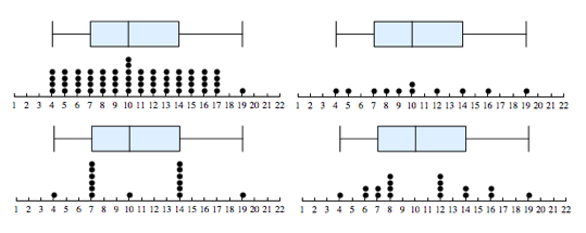
How are these data sets similar? Notice that the four data sets have the same boxplot. This is because the five-number summary is the same for each data set. The data sets have identical minimum value, maximum value, and quartile marks, so we could say that these data sets have the same center and spread.
- Center: Each data set has a median of 10.
- Spread: In each data set, the middle half of the data varies from 7 to 14, so the IQR is 7. In each data set, the data varies from 4 to 19, so the overall range is 15.
How are these data sets different? The data sets do not have the same number of data points. Also, the shape of each distribution is different.
The goal of the next Learn By Doing activity is to develop a deeper understanding of how the interquartile range (IQR) measures variability about the median. Use the simulation below for the next activity. You have used a similar simulation before. Recall the instructions for adding or removing data points:
- To add a point, move the slider to the value you want, then click Add.
- To remove a point, move the slider to the value you want, then click Minus.
- To reset the simulation, click the button in the upper left corner that says Reset.
Click here to open this simulation in its own window.
Learn By Doing
Candela Citations
- Concepts in Statistics. Provided by: Open Learning Initiative. Located at: http://oli.cmu.edu. License: CC BY: Attribution