Learning Objectives
- Find a confidence interval to estimate a population proportion when conditions are met. Interpret the confidence interval in context.
- Interpret the confidence level associated with a confidence interval.
A Look at 95% Confidence Intervals on the Number Line
Let’s look again at the formula for a 95% confidence interval.
[latex]\begin{array}{l}\mathrm{sample}\text{}\mathrm{statistic}\text{}±\text{}\mathrm{margin}\text{}\mathrm{of}\text{}\mathrm{error}\\ \mathrm{sample}\text{}\mathrm{proportion}\text{}±\text{}2(\mathrm{standard}\text{}\mathrm{errors})\end{array}[/latex]
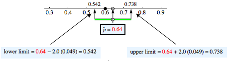
The lower end of the confidence interval is sample proportion – 2(standard error).
The upper end of the confidence interval is sample proportion + 2(standard error).
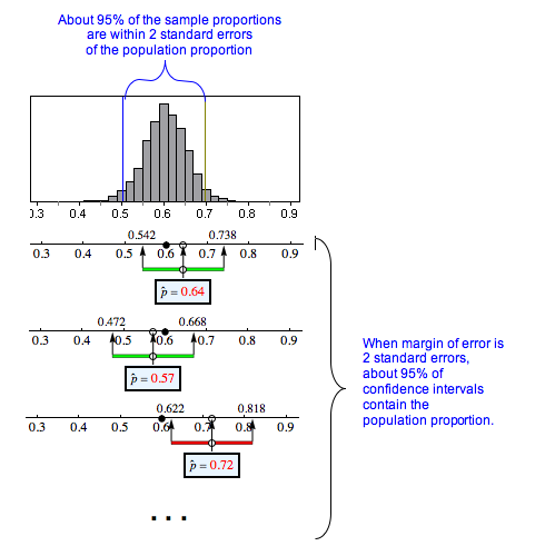
Every confidence interval defines an interval on the number line that is centered at the sample proportion. For example, suppose a sample of 100 part-time college students is 64% female. Here is the 95% confidence interval built around this sample proportion of 0.64.
We know the margin of error in a confidence interval comes from the standard error in the sampling distribution. For a 95% confidence interval, the margin of error is equal to 2 standard errors. This is shown in the following diagram.
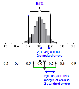
The width of the interval is the same as the width of the middle 95% of the sampling distribution. The next diagram illustrates this relationship.

When Does a 95% Confidence Interval Contain the True Population Proportion?
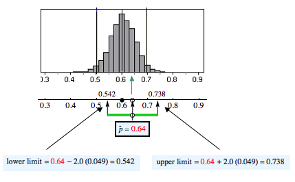
If the sample proportion has an error that is less than 2 standard errors, then the 95% confidence interval built around this sample proportion will contain the population proportion.
The sample proportion 0.64 is within 2 standard errors of 0.60, so 0.60 is in the 95% confidence interval built around 0.64.
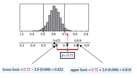
In the following figure, the sample proportion 0.72 is not within 2 standard errors of 0.60, so 0.60 is not in the 95% confidence interval built around 0.72.
How Confident Are We That a 95% Confidence Interval Contains the Population Proportion?
Following are three confidence intervals for estimating the proportion of part-time college students who are female. We are confident that most of these intervals will contain the population proportion, like the green intervals shown here. But some will not contain the population proportion, like the red interval shown here.
Of course, we don’t know the population proportion (which is why we want to estimate it with a confidence interval!). In reality, we cannot determine if a specific confidence interval does or does not contain the population proportion; that’s why we state a level of confidence. For these intervals, we are 95% confident that an interval contains the population proportion. In other words, 95% of random samples of this size will give confidence intervals that contain the population proportion. The sad news is that we never know if a particular interval does or does not contain the unknown population proportion.
Click here to open this simulation in its own window.
Learn By Doing
Connections to the Theoretical Sampling Distribution and Normal Model
For inference procedures, we work from a mathematical model of the sampling distribution instead of simulations. But we always begin our discussion with a simulation to highlight the sampling process. Simulations also remind us that the sampling distribution is a probability model because the sampling process is random and we look at long-run patterns.
Recall from “Distribution of Sample Proportions” our discussion of the mathematical model for the sampling distribution of sample proportions. For samples of size n, the model has the following center and spread, both of which are related to a population with a proportion p of successes.
Center: Mean of the sample proportions is p, the population proportion.
Spread: Standard deviation of the sample proportions (also called standard error) is [latex]\sqrt{\frac{p(1-p)}{n}}[/latex].
Shape: A normal model is a good fit for the sampling distribution if the expected number of successes and failures is at least 10. We can translate these conditions into formulas:
[latex]np≥10\text{}\mathrm{and}\text{}n(1-p)≥10[/latex]
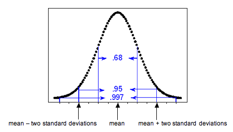
If we can use a normal model for the sampling distribution, then the empirical rule applies. Recall the empirical rule from Probability and Probability Distributions, which tells us the percentage of values that fall 1, 2, and 3 standard deviations from the mean in a normal distribution.
- 68% of the values fall within 1 standard deviation of the mean.
- 95% of the values fall within 2 standard deviations of the mean.
- 99.7% of the values fall within 3 standard deviations of the mean.
When we have a normal model for the sampling distribution, the mean of the sampling distribution is the population proportion. These ideas translate into the following statements:
- 68% of the sample proportions fall within 1 standard error of the population proportion.
- 95% of the sample proportions fall within 2 standard errors of the population proportion.
- 99.7% of the sample proportions fall within 3 standard errors of the population proportion.
Therefore, the empirical rule tells us that there is a 95% chance that sample proportions are within 2 standard errors of the population proportion. A margin of error equal to 2 standard errors, then, will produce an interval that contains the population proportion 95% of the time. In other words, we will be right 95% of the time. Five percent of the time, the confidence interval will not contain the population proportion, and we will be wrong. We can make similar statements for the other confidence levels, but these are less common in practice. For now, we focus on the 95% confidence level.
With the formula for the standard error, we can write a formula for the margin of error and for the 95% confidence interval:
[latex]\begin{array}{l}\mathrm{sample}\text{}\mathrm{statistic}\text{}±\text{}\mathrm{margin}\text{}\mathrm{of}\text{}\mathrm{error}\\ \mathrm{sample}\text{}\mathrm{proportion}\text{}±\text{}2(\mathrm{standard}\text{}\mathrm{error})\\ \stackrel{ˆ}{p}\text{}±\text{}2\sqrt{\frac{p(1-p)}{n}}\end{array}[/latex]
Remember that we can make a statement about our confidence that this interval contains the population proportion only when a normal model is a good fit for the sampling distribution of sample proportions.
Comment
You may realize that the formula for the confidence interval is a bit odd, since our goal in calculating the confidence interval is to estimate the population proportion, p. Yet the formula requires that we know p. For now, we use an estimate for p from a previous study when calculating the confidence interval. This is not the usual way statisticians estimate the standard error, but it captures the main idea and allows us to practice finding and interpreting confidence intervals. Later, we explore a different way to estimate standard error that is commonly used in statistical practice.
Example
Overweight Men
Recall the use of data from the National Health Interview Survey (conducted by the CDC) to estimate the prevalence of certain behaviors such as alcohol consumption, cigarette smoking, and hours of sleep for adults in the United States. In the 2005–2007 report, the CDC estimated that 68% of men in the United States are overweight. Suppose we select a random sample of 40 men this year and find that 75% are overweight. Using the estimate from the survey that 68% of U.S. men are overweight, we calculate the 95% confidence interval and interpret the interval in context.
Check normality conditions:
Yes, the conditions are met. The number of expected successes and failures in a sample of 40 are at least 10. We expect 68% of the 40 men to be overweight; [latex]np=40(0.68)[/latex] is about 27. We expect 32% of the 40 men to not be overweight; [latex]np=40(0.32)[/latex] is about 13.
We can use a normal model to estimate that 95% of the time a confidence interval with a margin of error equal to 2 standard errors will contain the proportion of overweight men in the United States this year.
Calculate the standard error (estimated average amount of error):
[latex]\mathrm{standard}\text{}\mathrm{error}=\sqrt{\frac{0.68(0.32)}{40}}\text{}\approx \text{}0.074[/latex]
Find the 95% confidence interval:
[latex]\begin{array}{l}\mathrm{sample}\text{}\mathrm{proportion}\text{}±\text{}\mathrm{margin}\text{}\mathrm{of}\text{}\mathrm{error}\\ 0.75\text{}±\text{}2(\mathrm{standard}\text{}\mathrm{error})\\ 0.75\text{}±\text{}2(0.074)\\ 0.75\text{}±\text{}0.148\\ 0.602\text{}\mathrm{to}\text{}0.898\end{array}[/latex]
Interpretation:
We are 95% confident that between 60.2% and 89.8% of U.S. men are overweight this year.
Learn By Doing
Learn By Doing
Candela Citations
- Concepts in Statistics. Provided by: Open Learning Initiative. Located at: http://oli.cmu.edu. License: CC BY: Attribution