Learning Outcomes
- Graph exponential growth and decay functions.
- Use the compound interest formula.
- Solve problems involving radioactive decay, carbon dating, and half life.
- Use Newton’s Law of Cooling.
- Use a logistic growth model.
- Choose an appropriate model for data.
We have already explored some basic applications of exponential and logarithmic functions. In this section, we explore some important applications in more depth including radioactive isotopes and Newton’s Law of Cooling.
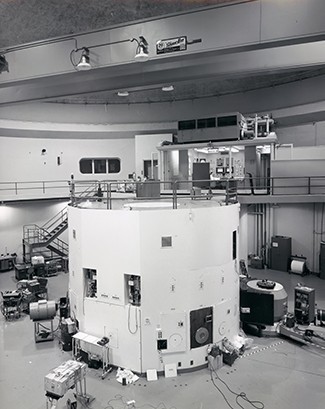
A nuclear research reactor inside the Neely Nuclear Research Center on the Georgia Institute of Technology campus. (credit: Georgia Tech Research Institute)
Exponential Growth and Decay
In real-world applications, we need to model the behavior of a function. In mathematical modeling, we choose a familiar general function with properties that suggest that it will model the real-world phenomenon we wish to analyze. In the case of rapid growth, we may choose the exponential growth function:
[latex]y={A}_{0}{e}^{kt}[/latex]
where [latex]{A}_{0}[/latex] is equal to the value at time zero, e is Euler’s constant, and k is a positive constant that determines the rate (percentage) of growth. We may use the exponential growth function in applications involving doubling time, the time it takes for a quantity to double. Such phenomena as wildlife populations, financial investments, biological samples, and natural resources may exhibit growth based odn a doubling time. In some applications, however, as we will see when we discuss the logistic equation, the logistic model sometimes fits the data better than the exponential model.
On the other hand, if a quantity is falling rapidly toward zero, without ever reaching zero, then we should probably choose the exponential decay model. Again, we have the form [latex]y={A}_{0}{e}^{-kt}[/latex] where [latex]{A}_{0}[/latex] is the starting value, and e is Euler’s constant. Now k is a negative constant that determines the rate of decay. We may use the exponential decay model when we are calculating half-life, or the time it takes for a substance to exponentially decay to half of its original quantity. We use half-life in applications involving radioactive isotopes.
In our choice of a function to serve as a mathematical model, we often use data points gathered by careful observation and measurement to construct points on a graph and hope we can recognize the shape of the graph. Exponential growth and decay graphs have a distinctive shape, as we can see in the graphs below. It is important to remember that, although parts of each of the two graphs seem to lie on the x-axis, they are really a tiny distance above the x-axis.
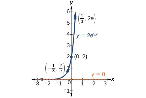
A graph showing exponential growth. The equation is [latex]y=2{e}^{3x}[/latex].
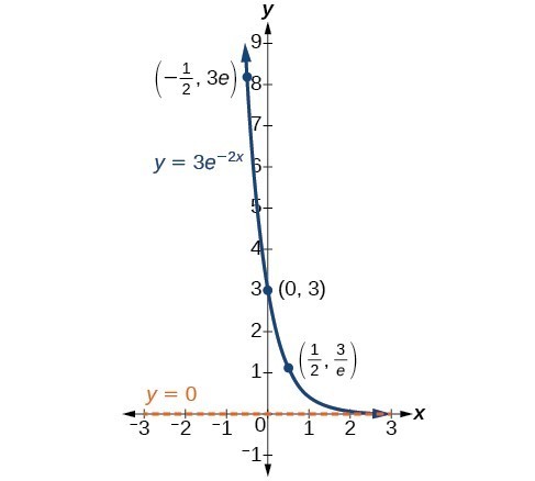
A graph showing exponential decay. The equation is [latex]y=3{e}^{-2x}[/latex].
Exponential growth and decay often involve very large or very small numbers. To describe these numbers, we often use orders of magnitude. The order of magnitude is the power of ten when the number is expressed in scientific notation with one digit to the left of the decimal. For example, the distance to the nearest star, Proxima Centauri, measured in kilometers, is 40,113,497,200,000 kilometers. Expressed in scientific notation, this is [latex]4.01134972\times {10}^{13}[/latex]. We could describe this number as having order of magnitude [latex]{10}^{13}[/latex].
A General Note: Characteristics of the Exponential Function [latex]y=A_{0}e^{kt}[/latex]
An exponential function of the form [latex]y={A}_{0}{e}^{kt}[/latex] has the following characteristics:
- one-to-one function
- horizontal asymptote: y = 0
- domain: [latex]\left(-\infty , \infty \right)[/latex]
- range: [latex]\left(0,\infty \right)[/latex]
- x intercept: none
- y-intercept: [latex]\left(0,{A}_{0}\right)[/latex]
- increasing if k > 0
- decreasing if k < 0
An exponential function models exponential growth when k > 0 and exponential decay when k < 0.
Using the Compound Interest Formula
Savings instruments in which earnings are continually reinvested, such as mutual funds and retirement accounts, use compound interest. The term compounding refers to interest earned not only on the original value, but on the accumulated value of the account.
The annual percentage rate (APR) of an account, also called the nominal rate, is the yearly interest rate earned by an investment account. The term nominal is used when the compounding occurs a number of times other than once per year. In fact, when interest is compounded more than once a year, the effective interest rate ends up being greater than the nominal rate! This is a powerful tool for investing.
For example, observe the table below, which shows the result of investing $1,000 at 10% for one year. Notice how the value of the account increases as the compounding frequency increases.
| Frequency | Value after 1 year |
|---|---|
| Annually | $1100 |
| Semiannually | $1102.50 |
| Quarterly | $1103.81 |
| Monthly | $1104.71 |
| Daily | $1105.16 |
We can calculate compound interest using the compound interest formula which is an exponential function of the variables time t, principal P, APR r, and number of times compounded in a year n.
A General Note: The Compound Interest Formula
Compound interest can be calculated using the formula
[latex]A\left(t\right)=P{\left(1+\frac{r}{n}\right)}^{nt}[/latex]
where
- A(t) is the accumulated value of the account
- t is measured in years
- P is the starting amount of the account, often called the principal, or more generally present value
- r is the annual percentage rate (APR) expressed as a decimal
- n is the number of times compounded in a year
Example: Calculating Compound Interest
If we invest $3,000 in an investment account paying 3% interest compounded quarterly, how much will the account be worth in 10 years?
Try It
An initial investment of $100,000 at 12% interest is compounded weekly (use 52 weeks in a year). What will the investment be worth in 30 years?
Example: Using the Compound Interest Formula to Solve for the Principal
A 529 Plan is a college-savings plan that allows relatives to invest money to pay for a child’s future college tuition; the account grows tax-free. Lily wants to set up a 529 account for her new granddaughter and wants the account to grow to $40,000 over 18 years. She believes the account will earn 6% compounded semi-annually (twice a year). To the nearest dollar, how much will Lily need to invest in the account now?
Try It
Refer to the previous example. To the nearest dollar, how much would Lily need to invest if the account is compounded quarterly?
Example: Graphing Exponential Growth
A population of bacteria doubles every hour. If the culture started with 10 bacteria, graph the population as a function of time.

Calculating Doubling Time
For growing quantities, we might want to find out how long it takes for a quantity to double. As we mentioned above, the time it takes for a quantity to double is called the doubling time.
Given the basic exponential growth equation [latex]A={A}_{0}{e}^{kt}[/latex], doubling time can be found by solving for when the original quantity has doubled, that is, by solving [latex]2{A}_{0}={A}_{0}{e}^{kt}[/latex].
The formula is derived as follows:
[latex]\begin{array}{l}2{A}_{0}={A}_{0}{e}^{kt}\hfill & \hfill \\ 2={e}^{kt}\hfill & \text{Divide both sides by }{A}_{0}.\hfill \\ \mathrm{ln}2=kt\hfill & \text{Take the natural logarithm of both sides}.\hfill \\ t=\frac{\mathrm{ln}2}{k}\hfill & \text{Divide by the coefficient of }t.\hfill \end{array}[/latex]
Thus the doubling time is
[latex]t=\frac{\mathrm{ln}2}{k}[/latex]
Example: Finding a Function That Describes Exponential Growth
According to Moore’s Law, the doubling time for the number of transistors that can be put on a computer chip is approximately two years. Give a function that describes this behavior.
Try It
Recent data suggests that, as of 2013, the rate of growth predicted by Moore’s Law no longer holds. Growth has slowed to a doubling time of approximately three years. Find the new function that takes that longer doubling time into account.
Half-Life
We now turn to exponential decay. One of the common terms associated with exponential decay, as stated above, is half-life, the length of time it takes an exponentially decaying quantity to decrease to half its original amount. Every radioactive isotope has a half-life, and the process describing the exponential decay of an isotope is called radioactive decay.
To find the half-life of a function describing exponential decay, solve the following equation:
[latex]\frac{1}{2}{A}_{0}={A}_{o}{e}^{kt}[/latex]
We find that the half-life depends only on the constant k and not on the starting quantity [latex]{A}_{0}[/latex].
The formula is derived as follows
[latex]\begin{array}{l}\frac{1}{2}{A}_{0}={A}_{o}{e}^{kt}\hfill & \hfill \\ \frac{1}{2}={e}^{kt}\hfill & \text{Divide both sides by }{A}_{0}.\hfill \\ \mathrm{ln}\left(\frac{1}{2}\right)=kt\hfill & \text{Take the natural log of both sides}.\hfill \\ -\mathrm{ln}\left(2\right)=kt\hfill & \text{Apply properties of logarithms}.\hfill \\ -\frac{\mathrm{ln}\left(2\right)}{k}=t\hfill & \text{Divide by }k.\hfill \end{array}[/latex]
Since t, the time, is positive, k must, as expected, be negative. This gives us the half-life formula
[latex]t=-\frac{\mathrm{ln}\left(2\right)}{k}[/latex]
In previous sections, we learned the properties and rules for both exponential and logarithmic functions. We have seen that any exponential function can be written as a logarithmic function and vice versa. We have used exponents to solve logarithmic equations and logarithms to solve exponential equations. We are now ready to combine our skills to solve equations that model real-world situations, whether the unknown is in an exponent or in the argument of a logarithm.
One such application is in science, in calculating the time it takes for half of the unstable material in a sample of a radioactive substance to decay, called its half-life. The table below lists the half-life for several of the more common radioactive substances.
| Substance | Use | Half-life |
|---|---|---|
| gallium-67 | nuclear medicine | 80 hours |
| cobalt-60 | manufacturing | 5.3 years |
| technetium-99m | nuclear medicine | 6 hours |
| americium-241 | construction | 432 years |
| carbon-14 | archeological dating | 5,715 years |
| uranium-235 | atomic power | 703,800,000 years |
We can see how widely the half-lives for these substances vary. Knowing the half-life of a substance allows us to calculate the amount remaining after a specified time. We can use the formula for radioactive decay:
[latex]\begin{array}{l}A\left(t\right)={A}_{0}{e}^{\frac{\mathrm{ln}\left(0.5\right)}{T}t}\hfill \\ A\left(t\right)={A}_{0}{e}^{\mathrm{ln}\left(0.5\right)\frac{t}{T}}\hfill \\ A\left(t\right)={A}_{0}{\left({e}^{\mathrm{ln}\left(0.5\right)}\right)}^{\frac{t}{T}}\hfill \\ A\left(t\right)={A}_{0}{\left(\frac{1}{2}\right)}^{\frac{t}{T}}\hfill \end{array}[/latex]
where
- [latex]{A}_{0}[/latex] is the amount initially present
- T is the half-life of the substance
- t is the time period over which the substance is studied
- y is the amount of the substance present after time t
How To: Given the half-life, find the decay rate
- Write [latex]A={A}_{o}{e}^{kt}[/latex].
- Replace A by [latex]\frac{1}{2}{A}_{0}[/latex] and replace t by the given half-life.
- Solve to find k. Express k as an exact value (do not round).
Note: It is also possible to find the decay rate using [latex]k=-\frac{\mathrm{ln}\left(2\right)}{t}[/latex].
Example: Using the Formula for Radioactive Decay to Find the Quantity of a Substance
How long will it take for 10% of a 1000-gram sample of uranium-235 to decay?
Try It
How long will it take before twenty percent of our 1000-gram sample of uranium-235 has decayed?
Example: Finding the Function that Describes Radioactive Decay
The half-life of carbon-14 is 5,730 years. Express the amount of carbon-14 remaining as a function of time, t.
Try It
The half-life of plutonium-244 is 80,000,000 years. Find a function that gives the amount of carbon-14 remaining as a function of time measured in years.
Radiocarbon Dating
The formula for radioactive decay is important in radiocarbon dating which is used to calculate the approximate date a plant or animal died. Radiocarbon dating was discovered in 1949 by Willard Libby who won a Nobel Prize for his discovery. It compares the difference between the ratio of two isotopes of carbon in an organic artifact or fossil to the ratio of those two isotopes in the air. It is believed to be accurate to within about 1% error for plants or animals that died within the last 60,000 years.
Carbon-14 is a radioactive isotope of carbon that has a half-life of 5,730 years. It occurs in small quantities in the carbon dioxide in the air we breathe. Most of the carbon on Earth is carbon-12 which has an atomic weight of 12 and is not radioactive. Scientists have determined the ratio of carbon-14 to carbon-12 in the air for the last 60,000 years using tree rings and other organic samples of known dates—although the ratio has changed slightly over the centuries.
As long as a plant or animal is alive, the ratio of the two isotopes of carbon in its body is close to the ratio in the atmosphere. When it dies, the carbon-14 in its body decays and is not replaced. By comparing the ratio of carbon-14 to carbon-12 in a decaying sample to the known ratio in the atmosphere, the date the plant or animal died can be approximated.
Since the half-life of carbon-14 is 5,730 years, the formula for the amount of carbon-14 remaining after t years is
[latex]A\approx {A}_{0}{e}^{\left(\frac{\mathrm{ln}\left(0.5\right)}{5730}\right)t}[/latex]
where
- A is the amount of carbon-14 remaining
- [latex]{A}_{0}[/latex] is the amount of carbon-14 when the plant or animal began decaying.
This formula is derived as follows:
[latex]\begin{array}{l}\text{ }A={A}_{0}{e}^{kt}\hfill & \text{The continuous growth formula}.\hfill \\ \text{ }0.5{A}_{0}={A}_{0}{e}^{k\cdot 5730}\hfill & \text{Substitute the half-life for }t\text{ and }0.5{A}_{0}\text{ for }f\left(t\right).\hfill \\ \text{ }0.5={e}^{5730k}\hfill & \text{Divide both sides by }{A}_{0}.\hfill \\ \mathrm{ln}\left(0.5\right)=5730k\hfill & \text{Take the natural log of both sides}.\hfill \\ \text{ }k=\frac{\mathrm{ln}\left(0.5\right)}{5730}\hfill & \text{Divide both sides by the coefficient of }k.\hfill \\ \text{ }A={A}_{0}{e}^{\left(\frac{\mathrm{ln}\left(0.5\right)}{5730}\right)t}\hfill & \text{Substitute for }r\text{ in the continuous growth formula}.\hfill \end{array}[/latex]
To find the age of an object we solve this equation for t:
[latex]t=\frac{\mathrm{ln}\left(\frac{A}{{A}_{0}}\right)}{-0.000121}[/latex]
Out of necessity, we neglect here the many details that a scientist takes into consideration when doing carbon-14 dating, and we only look at the basic formula. The ratio of carbon-14 to carbon-12 in the atmosphere is approximately 0.0000000001%. Let r be the ratio of carbon-14 to carbon-12 in the organic artifact or fossil to be dated determined by a method called liquid scintillation. From the equation [latex]A\approx {A}_{0}{e}^{-0.000121t}[/latex] we know the ratio of the percentage of carbon-14 in the object we are dating to the percentage of carbon-14 in the atmosphere is [latex]r=\frac{A}{{A}_{0}}\approx {e}^{-0.000121t}[/latex]. We solve this equation for t, to get
[latex]t=\frac{\mathrm{ln}\left(r\right)}{-0.000121}[/latex]
How To: Given the percentage of carbon-14 in an object, determine its age
- Express the given percentage of carbon-14 as an equivalent decimal r.
- Substitute for r in the equation [latex]t=\frac{\mathrm{ln}\left(r\right)}{-0.000121}[/latex] and solve for the age, t.
Example: Finding the Age of a Bone
A bone fragment is found that contains 20% of its original carbon-14. To the nearest year, how old is the bone?
Try It
Cesium-137 has a half-life of about 30 years. If we begin with 200 mg of cesium-137, will it take more or less than 230 years until only 1 milligram remains?
Bounded Growth and Decay
Using Newton’s Law of Cooling
Exponential decay can also be applied to temperature. When a hot object is left in surrounding air that is at a lower temperature, the object’s temperature will decrease exponentially, leveling off as it approaches the surrounding air temperature. On a graph of the temperature function, the leveling off will correspond to a horizontal asymptote at the temperature of the surrounding air. Unless the room temperature is zero, this will correspond to a vertical shift of the generic exponential decay function. This translation leads to Newton’s Law of Cooling, the scientific formula for temperature as a function of time as an object’s temperature is equalized with the ambient temperature.
The formula is derived as follows:
[latex]\begin{array}{l}T\left(t\right)=A{b}^{ct}+{T}_{s}\hfill & \hfill \\ T\left(t\right)=A{e}^{\mathrm{ln}\left({b}^{ct}\right)}+{T}_{s}\hfill & \text{Properties of logarithms}.\hfill \\ T\left(t\right)=A{e}^{ct\mathrm{ln}b}+{T}_{s}\hfill & \text{Properties of logarithms}.\hfill \\ T\left(t\right)=A{e}^{kt}+{T}_{s}\hfill & \text{Rename the constant }c \mathrm{ln} b,\text{ calling it }k.\hfill \end{array}[/latex]
A General Note: Newton’s Law of Cooling
The temperature of an object, T, in surrounding air with temperature [latex]{T}_{s}[/latex] will behave according to the formula
[latex]T\left(t\right)=A{e}^{kt}+{T}_{s}[/latex]
where
- t is time
- A is the difference between the initial temperature of the object and the surroundings
- k is a constant, the continuous rate of cooling of the object
How To: Given a set of conditions, apply Newton’s Law of Cooling
- Set [latex]{T}_{s}[/latex] equal to the y-coordinate of the horizontal asymptote (usually the ambient temperature).
- Substitute the given values into the continuous growth formula [latex]T\left(t\right)=A{e}^{k}{}^{t}+{T}_{s}[/latex] to find the parameters A and k.
- Substitute in the desired time to find the temperature or the desired temperature to find the time.
Example: Using Newton’s Law of Cooling
A cheesecake is taken out of the oven with an ideal internal temperature of [latex]165^\circ\text{F}[/latex] and is placed into a [latex]35^\circ\text{F}[/latex] refrigerator. After 10 minutes, the cheesecake has cooled to [latex]150^\circ\text{F}[/latex]. If we must wait until the cheesecake has cooled to [latex]70^\circ\text{F}[/latex] before we eat it, how long will we have to wait?
Try It
A pitcher of water at 40 degrees Fahrenheit is placed into a 70 degree room. One hour later, the temperature has risen to 45 degrees. How long will it take for the temperature to rise to 60 degrees?
Example: Using the Logistic-Growth Model
An influenza epidemic spreads through a population rapidly at a rate that depends on two factors. The more people who have the flu, the more rapidly it spreads, and also the more uninfected people there are, the more rapidly it spreads. These two factors make the logistic model good for studying the spread of communicable diseases. And, clearly, there is a maximum value for the number of people infected: the entire population.
For example, at time t = 0 there is one person in a community of 1,000 people who has the flu. So, in that community, at most 1,000 people can have the flu. Researchers find that for this particular strain of the flu, the logistic growth constant is b = 0.6030. Estimate the number of people in this community who will have had this flu after ten days. Predict how many people in this community will have had this flu after a long period of time has passed.
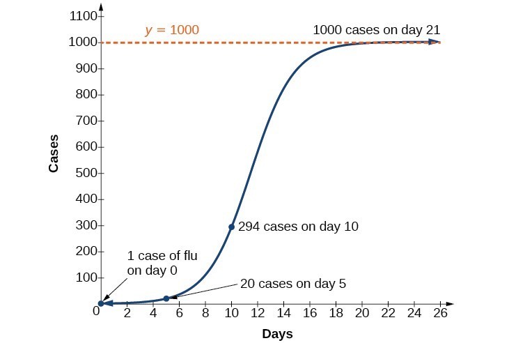
Try It
Using the model in the previous example, estimate the number of cases of flu on day 15.
Key Concepts
- The basic exponential function is [latex]f\left(x\right)=a{b}^{x}[/latex]. If b > 1, we have exponential growth; if 0 < b < 1, we have exponential decay.
- We can also write [latex]f\left(x\right)=a{b}^{x}[/latex] in terms of continuous growth as [latex]A={A}_{0}{e}^{kx}[/latex], where [latex]{A}_{0}[/latex] is the starting value. If [latex]{A}_{0}[/latex] is positive, then we have exponential growth when k > 0 and exponential decay when k < 0.
- We can use logistic growth functions to model real-world situations where the rate of growth changes over time, such as population growth, spread of disease, and spread of rumors.
- We can use real-world data gathered over time to observe trends. Knowledge of linear, exponential, logarithmic, and logistic graphs help us to develop models that best fit our data.
- Exponential growth functions are used to model situations where growth begins slowly and then accelerates rapidly without bound or where decay begins rapidly and then slows down to get closer and closer to zero.
Glossary
- carrying capacity
- in a logistic model, the limiting value of the output
- doubling time
- the time it takes for a quantity to double
- half-life
- the length of time it takes for a substance to exponentially decay to half of its original quantity
- logistic growth model
- a function of the form [latex]f\left(x\right)=\frac{c}{1+a{e}^{-bx}}[/latex] where [latex]\frac{c}{1+a}[/latex] is the initial value, c is the carrying capacity, or limiting value, and b is a constant determined by the rate of growth