Characteristics of Graphs of Logarithmic Functions
Before working with graphs, we will take a look at the domain (the set of input values) for which the logarithmic function is defined.
Recall that the exponential function is defined as [latex]y={b}^{x}[/latex] for any real number x and constant [latex]b>0[/latex], [latex]b\ne 1[/latex], where
- The domain of y is [latex]\left(-\infty ,\infty \right)[/latex].
- The range of y is [latex]\left(0,\infty \right)[/latex].
In the last section we learned that the logarithmic function [latex]y={\mathrm{log}}_{b}\left(x\right)[/latex] is the inverse of the exponential function [latex]y={b}^{x}[/latex]. So, as inverse functions:
- The domain of [latex]y={\mathrm{log}}_{b}\left(x\right)[/latex] is the range of [latex]y={b}^{x}[/latex]: [latex]\left(0,\infty \right)[/latex].
- The range of [latex]y={\mathrm{log}}_{b}\left(x\right)[/latex] is the domain of [latex]y={b}^{x}[/latex]: [latex]\left(-\infty ,\infty \right)[/latex].
Graphing a Logarithmic Function Using a Table of Values
Now that we have a feel for the set of values for which a logarithmic function is defined, we move on to graphing logarithmic functions. We begin with the function [latex]y={\mathrm{log}}_{b}\left(x\right)[/latex]. Because every logarithmic function of this form is the inverse of an exponential function of the form [latex]y={b}^{x}[/latex], their graphs will be reflections of each other across the line [latex]y=x[/latex]. To illustrate this, we can observe the relationship between the input and output values of [latex]y={2}^{x}[/latex] and its equivalent logarithmic form [latex]x={\mathrm{log}}_{2}\left(y\right)[/latex] in the table below.
| x | –3 | –2 | –1 | 0 | 1 | 2 | 3 |
| [latex]{2}^{x}=y[/latex] | [latex]\frac{1}{8}[/latex] | [latex]\frac{1}{4}[/latex] | [latex]\frac{1}{2}[/latex] | 1 | 2 | 4 | 8 |
| [latex]{\mathrm{log}}_{2}\left(y\right)=x[/latex] | –3 | –2 | –1 | 0 | 1 | 2 | 3 |
Using the inputs and outputs from the table above, we can build another table to observe the relationship between points on the graphs of the inverse functions [latex]f\left(x\right)={2}^{x}[/latex] and [latex]g\left(x\right)={\mathrm{log}}_{2}\left(x\right)[/latex].
| [latex]f\left(x\right)={2}^{x}[/latex] | [latex]\left(-3,\frac{1}{8}\right)[/latex] | [latex]\left(-2,\frac{1}{4}\right)[/latex] | [latex]\left(-1,\frac{1}{2}\right)[/latex] | [latex]\left(0,1\right)[/latex] | [latex]\left(1,2\right)[/latex] | [latex]\left(2,4\right)[/latex] | [latex]\left(3,8\right)[/latex] |
| [latex]g\left(x\right)={\mathrm{log}}_{2}\left(x\right)[/latex] | [latex]\left(\frac{1}{8},-3\right)[/latex] | [latex]\left(\frac{1}{4},-2\right)[/latex] | [latex]\left(\frac{1}{2},-1\right)[/latex] | [latex]\left(1,0\right)[/latex] | [latex]\left(2,1\right)[/latex] | [latex]\left(4,2\right)[/latex] | [latex]\left(8,3\right)[/latex] |
As we would expect, the x and y-coordinates are reversed for the inverse functions. The figure below shows the graphs of f and g.
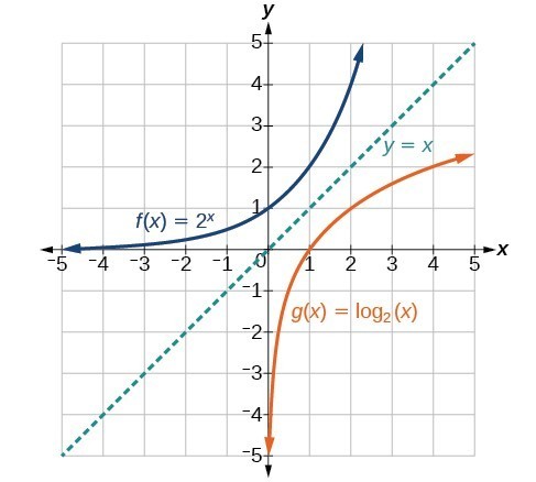
Notice that the graphs of [latex]f\left(x\right)={2}^{x}[/latex] and [latex]g\left(x\right)={\mathrm{log}}_{2}\left(x\right)[/latex] are reflections about the line y = x since they are inverses of each other.
Observe the following from the graph:
- [latex]f\left(x\right)={2}^{x}[/latex] has a y-intercept at [latex]\left(0,1\right)[/latex] and [latex]g\left(x\right)={\mathrm{log}}_{2}\left(x\right)[/latex] has an x-intercept at [latex]\left(1,0\right)[/latex].
- The domain of [latex]f\left(x\right)={2}^{x}[/latex], [latex]\left(-\infty ,\infty \right)[/latex], is the same as the range of [latex]g\left(x\right)={\mathrm{log}}_{2}\left(x\right)[/latex].
- The range of [latex]f\left(x\right)={2}^{x}[/latex], [latex]\left(0,\infty \right)[/latex], is the same as the domain of [latex]g\left(x\right)={\mathrm{log}}_{2}\left(x\right)[/latex].
Watch the following video for an excellent demonstration on how to graph a logarithmic function…
A General Note: Characteristics of the Graph of the Function [latex]f\left(x\right)={\mathrm{log}}_{b}\left(x\right)[/latex]
For any real number x and constant b > 0, [latex]b\ne 1[/latex], we can see the following characteristics in the graph of [latex]f\left(x\right)={\mathrm{log}}_{b}\left(x\right)[/latex]:
-
- one-to-one function
- vertical asymptote: x = 0
- domain: [latex]\left(0,\infty \right)[/latex]
- range: [latex]\left(-\infty ,\infty \right)[/latex]
- x-intercept: [latex]\left(1,0\right)[/latex] and key point [latex]\left(b,1\right)[/latex]
- y-intercept: none
- increasing if [latex]b>1[/latex]
- decreasing if 0 < b < 1
How To: Given a logarithmic function Of the form [latex]f\left(x\right)={\mathrm{log}}_{b}\left(x\right)[/latex], graph the function
- If the function is in function notation, replace [latex]f\left(x\right)[/latex] with y.
- Change the logarithmic equation to exponential form using the definition of the logarithm.
- Make a table of points, choosing the y-values first and finding the x-values, making sure to include the x-intercept.
- Plot the points. Make sure to include the x-intercept and the key point.
- Draw a smooth curve through the points.
- Draw and label the vertical asymptote.
Example: Graphing a Logarithmic Function Of the Form [latex]f\left(x\right)={\mathrm{log}}_{b}\left(x\right)[/latex]
Graph [latex]f\left(x\right)={\mathrm{log}}_{5}\left(x\right)[/latex]. State the domain, range, and asymptote.

Try It
Graph [latex]f\left(x\right)={\mathrm{log}}_{\frac{1}{5}}\left(x\right)[/latex]. State the domain, range, and asymptote.

The graphs below show how changing the base b in [latex]f\left(x\right)={\mathrm{log}}_{b}\left(x\right)[/latex] can affect the graphs. Observe that the graphs compress vertically as the value of the base increases. (Note: recall that the function [latex]\mathrm{ln}\left(x\right)[/latex] is base [latex]e\approx \text{2}.\text{718}[/latex] and [latex]\mathrm{log} (x)[/latex] is base 10.
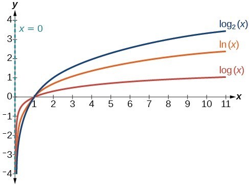
The graphs of three logarithmic functions with different bases all greater than 1.
Key Concepts
- The inverse of an exponential function is a logarithmic function, and the inverse of a logarithmic function is an exponential function.
- Logarithmic equations can be written in an equivalent exponential form using the definition of a logarithm.
- Exponential equations can be written in an equivalent logarithmic form using the definition of a logarithm.
- Logarithmic functions with base b can be evaluated mentally using previous knowledge of powers of b.
- Common logarithms can be evaluated mentally using previous knowledge of powers of 10.
- When common logarithms cannot be evaluated mentally, a calculator can be used.
- Natural logarithms can be evaluated using a calculator.
- To find the domain of a logarithmic function, set up an inequality showing the argument greater than zero and solve for x.
- The graph of the parent function [latex]f\left(x\right)={\mathrm{log}}_{b}\left(x\right)[/latex] has an x-intercept at [latex]\left(1,0\right)[/latex], domain [latex]\left(0,\infty \right)[/latex], range [latex]\left(-\infty ,\infty \right)[/latex], vertical asymptote x = 0, and
- if b > 1, the function is increasing.
- if 0 < b < 1, the function is decreasing.
Glossary
- common logarithm
- the exponent to which 10 must be raised to get x; [latex]{\mathrm{log}}_{10}\left(x\right)[/latex] is written simply as [latex]\mathrm{log}\left(x\right)[/latex]
- logarithm
- the exponent to which b must be raised to get x; written [latex]y={\mathrm{log}}_{b}\left(x\right)[/latex]
- natural logarithm
- the exponent to which the number e must be raised to get x; [latex]{\mathrm{log}}_{e}\left(x\right)[/latex] is written as [latex]\mathrm{ln}\left(x\right)[/latex]
Candela Citations
- Revision and Adaptation. Provided by: Lumen Learning. License: CC BY: Attribution
- Precalculus. Authored by: Jay Abramson, et al.. Provided by: OpenStax. Located at: http://cnx.org/contents/fd53eae1-fa23-47c7-bb1b-972349835c3c@5.175. License: CC BY: Attribution. License Terms: Download For Free at : http://cnx.org/contents/fd53eae1-fa23-47c7-bb1b-972349835c3c@5.175.
- College Algebra. Authored by: Abramson, Jay et al.. Provided by: OpenStax. Located at: http://cnx.org/contents/9b08c294-057f-4201-9f48-5d6ad992740d@5.2. License: CC BY: Attribution. License Terms: Download for free at http://cnx.org/contents/9b08c294-057f-4201-9f48-5d6ad992740d@5.2
- Questoin ID 34999, 35000. Authored by: Smart, Jim. License: CC BY: Attribution. License Terms: IMathAS Community License CC-BY + GPL
- Question ID 74340, 74341. Authored by: Nearing, Daniel. License: CC BY: Attribution. License Terms: IMathAS Community License CC-BY + GPL