what you’ll need to know
In this support activity you’ll become familiar with the following:
- Compare and contrast correlation coefficients among different scatterplots
- Compare the values of the correlation coefficient [latex]r[/latex] and the coefficient of determination [latex]R^{2}[/latex] for the same line.
- Use technology to explore the relationship between the correlation coefficient [latex]r[/latex] and coefficient of determination [latex]R^{2}[/latex] for a scatterplot.
- Use technology to explore the relationship between the sign of the slope, the spread and shape of the data, and the coefficient of determination [latex]R^{2}[/latex].
You will also have an opportunity to refresh the following skills:
- Express a proportion as a decimal and as a percentage.
- Determine the sign of a number that has been squared.
In the next preview assignment and in the next class, you will need to be able to express proportions as both decimals and percentages, understand what happens to a number when you square it, use technology to find the coefficient of determination ([latex]R^2[/latex]), and interpret [latex]R^2[/latex]. We’ll work through each of these skills in this corequisite support activity so that you’ll feel comfortable during the upcoming course activity.
This activity follows previous sections during which you built up a deep understanding of the components and processes of linear regression. See the first paragraph below and a reference list at the end of this page for a summary of those components and definitions.
The Correlation Coefficient and Related Operations
In previous activities, we examined ways of characterizing the linear relationship between two variables, including the correlation coefficient [latex]r[/latex] and the line of best fit. We will encounter an extension of these ideas here but first, let’s summarize what you’ve learned so far about linearly related bivariate data.
- In a linear relationship between two linked quantitative variables (bivariate data), the explanatory variable [latex]x[/latex] is the variable thought to explain or predict the response, and the response variable [latex]y[/latex] measured the outcome of interest, the response in the study. You may have seen these called the independent and dependent variables, [latex]x[/latex] and [latex]y[/latex] in a previous algebra class.
- it is common to represent the explanatory variable [latex]x[/latex] on the horizontal axis of a graph and the response variable [latex]y[/latex] on the vertical axis.
- The slope-intercept form of a linear equation is [latex]y=mx+b[/latex], where [latex]m[/latex] represents the slope, or constant rate of change in the relationship between variables, and [latex]b[/latex] represents the y-intercept, the point at which the input [latex]x=0[/latex] and where the line crosses the y-axis on the graph.
- The slope-intercept form of a linear equation is commonly expressed in statistics using [latex]\hat{y}= a + bx[/latex], where [latex]b[/latex] represents the constant rate of change and [latex]a[/latex] represents the y-intercept.
- We use a Least Squares Regression analysis to determine the equation of a line of best fit in order to make predictions based on an existing dataset.
- The line of best is a line that best describes a scatterplot of the data by minimizing the total vertical distances (errors) from all the data points to the line.
- The vertical error associated with each data point (the distance from the point to the line of best fit) is called the residual of that data point. It lets us know how far off the prediction made by the line of best fit is from the actual observation.
- The correlation coefficient [latex]r[/latex] describes the strength and direction of the linear relationship between the two quantitative variables in the dataset.
The Correlation Coefficient
In this activity, we want to begin to understand a new measure: the coefficient of determination. Like the correlation coefficient, this measure will reveal information about the linear relationship in bivariate data. Your goal in this activity will be to discover how the coefficient of determination is calculated and to start to understand what it says about the data.
Let’s begin by extending your understanding of the correlation coefficient in Question 1. Then in Questions 2 and 3, you’ll compare the correlation coefficient [latex]r[/latex] with the coefficient of determination [latex]R^{2}[/latex] for the same set of data points.
question 1
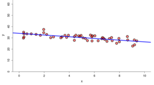
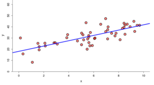
Consider the following examples of lines of best fit, including the correlation coefficients corresponding to each scatterplot. How are the plots similar and how are they different? The first scatterplot has [latex]r=-0.72[/latex], and the second scatterplot has [latex]r=0.75[/latex].
Correlation Coefficient vs. Coefficient of Determination
You’ve seen that the correlation coefficient [latex]r[/latex] is a measure of the strength and direction of a linear relationship. When interpreting the value of [latex]r[/latex], we should ask if the line of best fit for the data has a positive or negative slope and whether the data appear tightly correlated to the line.
In Question 2, you’ll compare [latex]r[/latex] with [latex]R^2[/latex] for the same data. As you do, try to develop your own understanding of how the two measures relate, then express that understanding to answer Question 3.
Note that the coefficient of determination may be expressed either as [latex]R^{2}[/latex] or [latex]r^{2}[/latex].
question 2
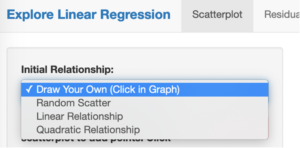
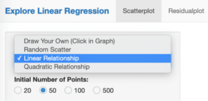
Go to the Explore Linear Regression tool at https://dcmathpathways.shinyapps.io/ExploreLinReg/. From the drop-down menu, select “Linear Relationship.”
From the drop-down menu, select “Draw Your Own (Click in Graph).”
Part A: As we have seen before (and as the term “line of best fit” implies), linear regression can be an appropriate model when the scatterplot of a dataset shows a linear trend in the relationship between the explanatory variable and the response variable.
By clicking on the graph, create a scatterplot with at least five data points that lie on (or very close to) a line with non-zero slope.
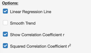
Check the boxes for “Linear Regression Line,” “Show Correlation Coefficient [latex]r[/latex],” and “Squared Correlation Coefficient [latex]r^2[/latex].”
Look at the table below the scatterplot. What is the value of the correlation coefficient? What is the value of the coefficient of determination?
Part B: Reset the scatterplot by clicking the red “Reset” button. Now, click on the graph to create a scatterplot with at least five data points that lie near (but not on) a line with non-zero slope.
What is the value of the correlation coefficient? What is the value of the coefficient of determination?
Part C: Reset the scatterplot by clicking the red “Reset” button. Now, click on the graph to create a scatterplot with at least five arbitrarily-placed data points.
What is the value of the coefficient of determination?
question 3
Based on your answer to the previous question, what do you notice about the relationship between the correlation coefficient and the coefficient of determination?
Coefficient of Determination
Question 4 refers to the sign of a number. Recall that the sign of a number tells you whether that number is positive or negative. For example, the sign of the number -3 is negative, while the sign of the number 77 is positive.
question 4
From the drop-down menu, select “Linear Relationship.”
Explore this page by changing different settings and use your observations to answer the following questions.
Part A: Does the sign of the coefficient of determination depend on the sign of the slope of the linear relationship?
Part B: How does the spread of the data away from the line of best fit affect the coefficient of determination?
question 5
Based on your observations, what do you think the coefficient of determination tells us?
The coefficient of determination, denoted [latex]R^2[/latex] and pronounced “R squared,” is the proportion of the variation in the response variable that can be explained by its linear relationship with the explanatory variable. Some people prefer to use the symbol [latex]r^2[/latex] (like in the DCMP Data Analysis Tools), but [latex]R^2[/latex] and [latex]r^2[/latex] mean the same thing. In this course, we will use the notation [latex]R^2[/latex]. In the preview assignment and in-class activity, we will discuss the coefficient of determination in more detail. For now, our goal is to lay the groundwork in order to be prepared for those activities coming up.
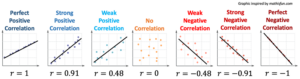
The reason that we use this symbol is that the coefficient of determination is equal to the square of the correlation coefficient. Because of this, [latex]R^2[/latex] is more sensitive to differences in the strength of the linear relationship between the two variables than [latex]r[/latex] is. This increased sensitivity can be seen in the following graphic; the difference between [latex]R^2[/latex] values is greater than the difference between corresponding [latex]r[/latex] values.
Decimals and Percentages
Recall
See the Student Resource[Fractions, Decimals, Percentages] for a refresher on converting decimals to percentages and vice-versa.
Practice converting between decimals and percentages in Question 6 before moving on.
question 6
Depending on the tools you use, [latex]R^2[/latex] may be expressed as a decimal or as a percentage. Even though the tool expresses [latex]R^2[/latex] as a percentage, it is important to be able to convert between the two forms.
If you are given a number as a decimal and want to convert it to a percentage, multiply the number by 100 and use the % symbol afterward. For example, the decimal [latex]0.489[/latex] is converted to a percentage as follows:
[latex]0.489 \rightarrow 0.489 \times 100 \% \rightarrow 48.9 \%[/latex]
If you are given a number as a percentage and want to convert it to a decimal, divide the percentage by 100 and remove the % symbol. For example, the percentage [latex]67\%[/latex] is converted to a decimal as follows:
[latex]67 \% \rightarrow 67\div 100\rightarrow 0.67[/latex]
For each of the following, if you are given a decimal, convert it to a percentage. If you are given a percentage, convert it to a decimal.
Hint: To multiply a number by 100, move the decimal in the number two places to the right. To divide a number by 100, move the decimal two places to the left.
Ex. [latex]0.3 \times 100 = 30.0[/latex]
Ex. [latex]5 \div 100 = 0.05[/latex]
Part A: [latex]0.4[/latex]
Part B: [latex]1[/latex]
Part C: [latex]36\%[/latex]
Part D: [latex]2.1[/latex]
Part E: [latex]55.7\%[/latex]
Squaring Numbers
Since the coefficient of determination is equal to the square of the correlation coefficient, we will examine the operation of squaring. Squaring a number is the same as multiplying that number by itself. For example,
[latex]5^2=5\cdot 5=25[/latex]
[latex](-2)^2=(-2)\cdot (-2)=4[/latex]
[latex]1^2=1\cdot 1=1[/latex]
question 7
What can you say about the sign of a number that has been obtained through squaring?
Do you suppose it may be true that squaring a number always yields a larger number as in the examples above? Let’s explore that idea by trying to find an example in which squaring a number yields either a smaller or the same number in return.
A counterexample is an example that contradicts or disproves a general statement. For instance, suppose someone proposes the following general statement:
“All people like ice cream.”
A counterexample to this statement would be someone who doesn’t like ice cream. It only takes one counterexample to show that a statement is false.
question 8
Someone makes the claim that squaring a number always makes it bigger. Find a counterexample to disprove their claim.
Question 9 will help you make sense of what happens when a number is squared.
question 9
We can use an area model to see why the previous claim is false.
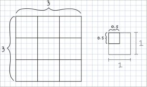
Part A: What expression is represented in the model on the left? Simplify this expression.
Part B: What expression is represented in the model on the right? Simplify this expression.
Part C: Why does squaring 0.5 result in a number that is smaller than 0.5?
question 10
Using what you know about what happens when you square a number, explain your answers to Question 3 and Question 4, Part A.
question 11
For what values of [latex]r[/latex] will [latex]r=R^2[/latex]? Explain your reasoning using what you know about squaring and what you know about the meaning of [latex]r[/latex] and [latex]R^2[/latex].
Now that you have a good sense of what happens mathematically when calculating the coefficient of determination, let’s return to the data analysis tool in Questions 12, 13, and. Use the knowledge you gained during this activity to create scatterplots that demonstrate a particular coefficient of determination.
question 12
Using what you now know about [latex]R^2[/latex], use the Explore Linear Regression tool to create a scatterplot with a very small value for [latex]R^2[/latex].
question 13
Building on this, use the Explore Linear Regression tool to create a scatterplot with a very small value for [latex]R^2[/latex] but also with some kind of pattern to the scatterplot (in other words, the points aren’t just randomly placed).
Now consider the similarities and differences in the plots you created in Questions 12 and 13. What led to [latex]R^{2}[/latex] being so small in these cases? What other information might we need to besides [latex]r[/latex] and [latex]R^{2}[/latex] to make decisions about the appropriateness of fitting a line? Use this line of thought to answer Question 14.
question 14
Determine whether the following statement is true or false, and if it is false, provide a counterexample: “If [latex]R^2[/latex] is very small, that means there is no relationship between the explanatory variable and the response variable.”
You’ve learned in depth about bivariate regression analysis over the past several sections of the course and will continue this exploration during the upcoming material and activity as you gain a deeper understanding of [latex]R^{2}[/latex]. You can return to the following sections as needed to refresh these ideas:
- [Section 5A]: bivariate data, scatterplots, trends, correlation coefficient.
- [Section 6A]: constant rates of change, graphs, explanatory and response variables, Least Squares Regression analysis, linear modeling, residuals, line of best fit, linear equation, y-intercept, slope.
- [Section 6B]: calculating slope as rise over run, graphing lines using slope and y-intercept, mathematical models, statistical models, estimated y-intercept and estimated slope, extrapolation.
- [Section 6C]: understanding and interpreting the correlation coefficient, the coefficient of determination.
In the following section, [6D], you’ll explore an extension of residuals and then put all of your understanding together in [6E] to perform an entire analysis of bivariate data.
Let’s move on to the course material and activity for this section now.
