Learning Goals
At the end of this page, you should feel comfortable performing these skills:
- Calculate and interpret residual errors.
- Identify violations of assumptions needed to perform linear regression.
- Discuss the effect of influential points on [latex]R^{2}[/latex].
In the next in-class activity, you will need to calculate and interpret residuals, identify violations of the assumptions needed to perform linear regression, and discuss the effect of outliers on [latex]R^2[/latex]. Let’s prepare for that by learning the formula for calculating residuals, seeing how to interpret a residual error for an observed value, and then challenging assumptions about the appropriateness of linear regression from the perspective of residuals. We’ll end this preparation assignment with a discussion on how outliers affect the coefficient of determination.
Residual Error
We have used scatterplots of data and constructed lines of best fit to describe the relationship in bivariate data. You have learned about the correlation coefficient [latex]r[/latex] and the coefficient of determination [latex]R^2[/latex], which are tools we have for determining whether the line of best fit is a useful model and how well the line fits the data.
Calculation and Interpretation
Another tool we have is the analysis of residuals, which you saw for the first time in In-Class Activity 6.A. When we fit a line to the data, one thing we are interested in is how similar the linear model’s predictions are to the observed data—in other words, we want to know how closely the model matches the data. The residual for a data point is the difference between the observed value of the response variable and the linear model’s prediction.
Residual = observed value – predicted value
Residual = [latex]y-\hat y[/latex]
To calculate the predicted value, input a value of the explanatory variable, [latex]x[/latex], to get a predicted value of the response variable, [latex]\hat y[/latex]. For example, suppose you have the following equation:
[latex]\hat y=5+3.4x[/latex].
You can calculate the predicted value of the response variable for a value of the explanatory variable [latex]x=6[/latex] in the following way:
[latex]\hat y=5+3.4\cdot 6=5+20.4=25.4[/latex]
Thus, when [latex]x=6[/latex], the predicted value of [latex]\hat y[/latex] will be 20.4.
See the video below for a demonstration before attempting Question 1.
Video Placement
[Worked example video: A video following the process above to calculate a residual error. It should preview questions similar to the ones in Question 1 belos.]
Now you try calculating and interpreting residuals in Question 1.
Question 1
Consider the following scatterplot, with the equation of the line of best fit given in the upper left corner. This dataset has compiled information about 21 different animal species and recorded the average longevity (or lifespan) in years of each animal, along with the animal’s average gestational period (how long a fetus must develop before it is born) in days. We will pay particular attention to the observation corresponding to the bear.
The equation of the line of best fit is:
[latex]\hat y=6.29+0.0449x[/latex]
There is text on the scatterplot that reads:
Animal: Bear
Gestation (days): 220
Longevity (years): 22
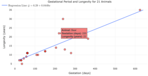
Part A: The bear’s average gestational period is 220 days. What is the bear’s predicted average longevity in years given by the line of best fit?
Part B: What is the bear’s actual average longevity in years?
Part C: What is the residual for the observation corresponding to the bear?
Part D: Interpret the meaning of the residual by filling in the blanks:
The bear’s actual longevity is _____ years greater/less than predicted.
In the case of the bear, we saw that the residual for the observation was a positive number and that the data point was located above the line of best fit. What would happen to the sign of the residual if the data point were to lie below the line of best fit?
Example
As you saw in the text and video demonstration above, use the formula given to calculate the residual error for
an observed value of the response variable, where [latex]y[/latex] represents the observed value and [latex]\hat{y}[/latex] represents the predicted value.
[latex]y - \hat{y}=\text{residual}[/latex]
Calculate the following residuals for the statistical model given in Question 1: [latex]\hat{y} = 6.29 + 0.0449x[/latex].
- The observed data point lies at (260, 30). What is the residual for this observation? Does the data point lie above or below the line of best fit?
- The observed data point lies at (290, 8). What is the residual for this observation? Does the data point lie above or below the line of best fit?
- The observed data point lies at (65, 9). What is the residual for this observation? Does the data point lie above or below the line of best fit?
Now that you've seen examples of residuals for data points above, below, and very close to the line of best fit, use what you know to answer Questions 2, 3, and 4 below.
question 2
Fill in the blank: If a residual error is positive, then the observed value is ______ the predicted value.
- a) Greater than
- b) Less than
- c) Equal to
question 3
Fill in the blank: If a residual is negative, then the observed value is ______ the predicted value.
- a) Greater than
- b) Less than
- c) Equal to
question 4
Which feature on the following scatterplot represents the residuals?
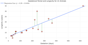
- a) The blue line
- b) The vertical green lines
- c) The red dots
Necessary Assumptions
Examining the residuals can give us useful information about whether a line of best fit is an appropriate choice to model the data in question.
Video Placement
[Perspective Video: a 3-instructor video presenting and annotating examples of scatterplots in which the residuals indicate the data is appropriate for a linear model, then also showing plots inappropriate for linear analysis that violate the necessary conditions in the ways indicated below. This presentation should be more intuitive and visual than technical but it may include technical discussion presented in the text above. ]
When a linear regression is appropriate, the value of the residuals will be randomly scattered around 0. That is, some residuals will be positive (observed value above the line) and some will be negative (observed value below the line), but we do not want to see some systematic pattern (e.g., all above in order and then all below).
In particular, we might worry about the appropriateness of the model if we notice the following:
- The trend in the scatterplot is non-linear, indicating that the relationship between the explanatory variable and the response variable is not modeled very well by a line. The residuals tend to have a pattern. The observations are above and below the line systematically.
- The observed values are further and further away from the line of best fit for a portion of the data. That is, the errors are not consistent for all values of the explanatory variable. Often, we will see that the size of the residuals tends to increase or decrease as the value of the explanatory variable increases. When this happens, it can be hard to get a handle on the accuracy of the model because the standard deviation of the residuals is not constant over the values of the independent variable.
Consider the conditions required for using a line to model data (listed in the text and the video above) as you explore scenarios of scatterplots in which one of those conditions has been violated.
question 5
For each of the following examples, one of our necessary conditions has been violated. Indicate how you know a condition has been violated.
Part A:
How do you know a condition has been violated?
- a) The trend in the scatterplot is non-linear.
- b) The size of the residuals tends to increase or decrease as the value of the explanatory variable increases.
Part B:
How do you know a condition has been violated?
- a) The trend in the scatterplot is non-linear.
- b) The size of the residuals tends to increase or decrease as the value of the explanatory variable increases.
Outliers
We also might worry about the appropriateness of the model if we notice an extreme observation that affects the value of the line. Recall from earlier activities that an outlier is an extreme observation that is far away from the rest of the data. In fitting a regression line, an outlier can also be an observation that does not fit the trend of the data as well. We call this type of outlier an influential point. This point drastically changes the equation of the line, consequently increasing the values of all of the residuals. An influential point appears to “pull” the line towards its value. We will also study how these points affect [latex]R^2[/latex]. It is important to note that not all outliers affect the equation of the line, so we will need to investigate.
Example
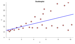
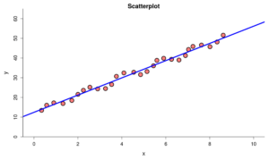
Recall that an outlier is an extreme observation far away from the rest of the data. Observe the two scatterplots below. Both contain 19 identical data points but the second plot contains an influential point. Notice the effect the outlier has on the regression line.
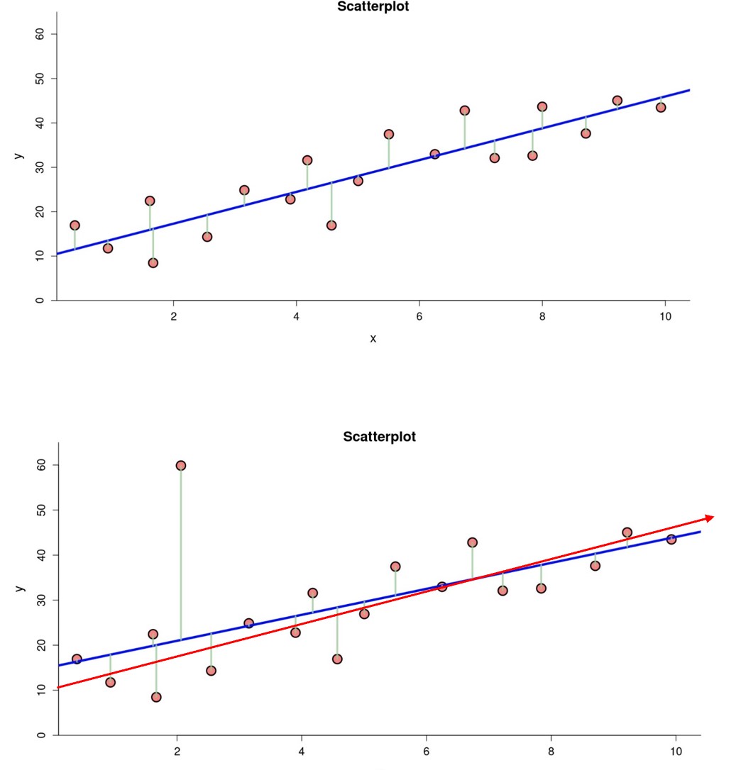
The red line in the second plot is the original line of best fit. The extreme outlier appears to have pulled the line upward in the second plot.
- What is the y-intercept in the first plot, without the outlier?
- What is the y-intercept in the second plot, with the extreme outlier?
Note the differences in the characteristics of the two lines.
| Slope | [latex]r[/latex] | [latex]R^{2}[/latex] | |
| Original line without the outlier | [latex]3.84[/latex] | [latex]0.90[/latex] | [latex]81 \%[/latex] |
| Second line with the outlier | [latex]3.84[/latex] | [latex]0.64[/latex] | [latex]40 \%[/latex] |
As we noted above, not all outliers qualify as influential points. That is, not all outliers have a large effect on the slope of the regression line. Question 6 and 7 will help illustrate this idea.
question 6
Open the DCMP Linear Regression tool at https://dcmathpathways.shinyapps.io/LinearRegression/. Open the “Animal Longevity” dataset. This is the same dataset that was used in Question 1. Make sure that gestation is the explanatory variable and longevity is the response variable.
Part A: Find the point on the graph corresponding to the elephant by hovering over the points. Is this observation an outlier that does not fit the trend?
- a) Yes
- b) No
Part B: What is [latex]R^2[/latex] for this dataset?
Part C: Select the box on the left side of screen that says “Click to Remove Points.” Remove the point corresponding to the elephant by either clicking on the scatterplot or by highlighting the elephant row in the data table and deleting it. How does [latex]R^2[/latex] change when you remove the elephant from the dataset?
- a) [latex]R^2[/latex] increases
- b) [latex]R^2[/latex] decreases
- c) [latex]R^2[/latex] stays the same
Part D: Why do you think this is? How does removing the elephant affect the relative amount of variability that is explained by the linear relationship?
Question 7
Now, reload the “Animal Longevity” dataset so that the data for the elephant are included once again. You may need to reload the webpage, then reload the dataset.
Part A: Find the point on the graph corresponding to the hippopotamus. Is this observation an outlier?
- a) Yes
- b) No
Part B: What is [latex]R^2[/latex] for this dataset?
Part C: Select the box on the left side of screen that says “Click to Remove Points.” Remove the point corresponding to the hippopotamus by either clicking on the scatterplot or by highlighting the hippopotamus row in the data table and deleting it. How does [latex]R^2[/latex] change when you remove the hippopotamus from the dataset?
- a) [latex]R^2[/latex] increases
- b) [latex]R^2[/latex] decreases
- c) [latex]R^2[/latex] stays the same
Part D: Why do you think this is? How does removing the hippopotamus affect the relative amount of variability that is explained by the linear relationship?
Finally, let's move our attention from the idea of influential points to consider again the shape of a plot with respect to a very large or very small value of [latex]R^2[/latex]. Recall the situations you explored above that violate conditions necessary to consider a linear model appropriate for data. Then answer Question 8.
question 8
Consider this plot again, which we saw in a previous question. The scatterplot has [latex]R^2=98.2\%[/latex].
Determine whether the following statement is true or false: If the scatterplot of two variables has a high [latex]R^2[/latex] value, then a line is an appropriate model for the relationship between the variables.
Summary
In this What to Know page, you calculated and interpreted residuals and examined assumptions and the effects of outliers on the appropriateness of a linear model for bivariate data. Let’s summarize these three ideas by noting the questions in which they appeared.
- In Questions 1, 2, 3, and 4, you calculated and interpreted residual errors.
- In Questions 5 and 8, you identified violations of assumptions needed to perform linear regression.
- In Questions 6 and 7, you discussed the effect of influential points on [latex]R^{2}[/latex].
Understanding the characteristics and processes of analyzing residuals is crucial to performing linear regression analysis on data. Let's move on to the activity to apply these skills.
