Preparing for the next class
In the next in-class activity, you will need to use the correct notation to identify elements of a binomial experiment, compute the mean and standard deviation of a binomial random variable, and use technology to calculate binomial probabilities. You will also need to determine whether a probability experiment has a binomial distribution and describe the shape of a distribution.
In In-Class Activity 8.C, we defined a binomial experiment as an experiment consisting of a fixed number, [latex]n[/latex], of independent Bernoulli trials that count the number of successes out of [latex]n[/latex] trials. Notice that the number of successes in a binomial experiment is a discrete random variable. The distribution of this random variable is modeled with the binomial distribution.
Binomial Distribution
For a binomial experiment, the mean and standard deviation are defined as follows:
- The mean of the number of successes is [latex]\mu = np[/latex].
- The standard deviation of the number of successes is [latex]\sigma = \sqrt{np(1-p)}[/latex].
Question 1
Common tests such as the SAT, ACT, LSAT, and MCAT use multiple-choice test questions with five possible answer choices (a, b, c, d, and e). In addition, each question has only one correct answer.
Let the random variable X represent the number of correct responses. For people who make random guesses for answers to a block of 100 questions, identify the values for [latex]p, 1-p,[/latex] mean of [latex]X[/latex], and standard deviation of [latex]X[/latex].
What do the mean and standard deviation measure in the context of this question?
Question 2
In the National Basketball Association (NBA), the top free throw shooters usually have a probability of about 0.90 of making any given free throw.
- During the 2020–21 season, Paul George of the LA Clippers was considered one of the top free throw shooters in the league. Suppose that in an upcoming game, George will attempt 9 free throws. [latex]Let X =[/latex] the number of free throws made. What must you assume for X to have a binomial distribution? Explain.
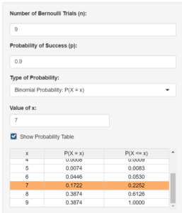
- Specify the values of [latex]n \mbox{ and } p[/latex]for the binomial distribution of [latex]X[/latex] in Part a.Go to the DCMP Binomial Distribution tool at https://dcmathpathways.shinyapps.io/BinomialDist/ and click on the Find Probabilities tab at the top of the page.Use the tool to answer the following questions.
- Find the probability that George makes all 9 free throws.
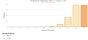
- Describe the shape of the distribution for the scenario in Part c.
- Bell shaped
- Skewed right
- Skewed left
- Uniform
- Probability that George makes more than 6 free throws.
- Suppose that over the course of a season, George will shoot 300 free throws. Let’s treat the 300 free throws as [latex]trials. Calculate the probability that George makes at least 268 free throws.
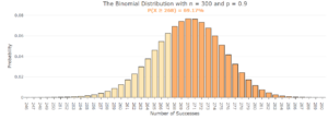
- Describe the shape of the distribution for the scenario in Part f.
- Bell shaped
- Skewed right
- Skewed left
- Uniform
Oftentimes, it is adequate to use the mean and standard deviation to describe the most likely values for the number of successes. For large [latex] n~(\mbox{when}~np\geq 10 \mbox{ and } n(1 – p) \geq 10)[/latex], the binomial distribution has an approximate bell shape. So, we can use the normal distribution to approximate the binomial distribution and conclude that nearly all possibilities for the number of successes fall between the mean and 3 standard deviations.
Question 3
Refer to the scenario regarding free throws made by Paul George over the course of a season where he will attempt 300 free throws. Let’s treat the 300 free throws as [latex]n = 300[/latex] trials. From the fact that the top free throw shooters make 90% of all free throws, we can deduce that they miss 10% of their free throws. We can assume that successive shots are independent. Under these assumptions, we can model the number of free throws made as a binomial distribution with [latex]n = 300 \mbox{ and } p = 0.90[/latex].
- To the nearest whole number, find the mean and standard deviation of the probability distribution of the number of free throws that are successes, [latex]X[/latex]. Then interpret these values.
Hint: Recall that the mean is [latex]\mu = np[/latex]. Remember, the mean can be interpreted as the expected value or anticipated value of [latex]X[/latex]. The standard deviation of [latex]X = \sqrt{np(1-p)}[/latex]. - According to the Empirical Rule, within what range would you expect the number of free throws made to almost certainly fall? Explain.Hint: Recall that the Empirical Rule states that 99.7% of the values will fall within 3 standard deviations of the mean.
- Within what range would you expect the proportion of free throws made to fall almost certainly?Hint: The endpoints for the ranges can be used to calculate the proportion.
Question 4
Use the DCMP Binomial Distribution tool to answer the following questions.
- Under the Explore tab, move the slider for [latex]p[/latex] to 0.2 and move the slider for [latex]n[/latex] to 10. Draw a quick sketch of the distribution in your notes and then select the following best choice that describes the shape of the distribution.
- Bell shaped
- Skewed right
- Bi-modal
- Skewed left
- Next, set [latex]p = 0.2[/latex] and [latex]n= 30[/latex]. Draw a quick sketch of the distribution in your notes and then select the following best choice that describes the shape of the distribution.
- Symmetric
- Skewed right
- Bi-modal
- Skewed left
- Next, set [latex]p=0.2[/latex] and [latex]n= 70[/latex]. Draw a quick sketch of the distribution in your notes and then select the following best choice that describes the shape of the distribution.
- Symmetric
- Skewed right
- Bi-modal
- Skewed left
- Which continuous probability distribution does the graph in Part c resemble?
- What role does latex] n [/latex] play in the shape of the binomial distribution?
