Preparing for the next class
In the next in-class activity, you will need to describe how the center, spread, and shape of a sampling distribution of a sample proportion varies with the sample size, [latex]n[/latex], and the population proportion, [latex]p[/latex]. You will also need to use a normal distribution to approximate probabilities and percentiles involving a sample proportion.
Go to the DCMP Sampling Distribution of the Sample Proportion tool at https://dcmathpathways.shinyapps.io/SampDist_Prop/.
We are going to use this tool to simulate sample proportions from samples of varying sizes, [latex]n[/latex], from populations with varying proportions, [latex]p[/latex]. Make sure to:
- Leave the default values for the population proportion ([latex]p[/latex]) and the sample size ([latex]n[/latex]).
- Select 1,000 and click “Draw Samples” to generate sample proportions from 1,000 random samples.
- Check the “Show Normal Approximation” option box. This will overlay a normal distribution on the distribution of sample proportions, which will allow you to compare how closely the simulated distribution follows a normal distribution.
The bottom plot in the tool, “Sampling Distribution of Sample Proportion,” now displays a plot of the distribution of these randomly generated sample proportions.
Question 1
Slide the “Population Proportion ([latex]p[/latex])” slider to explore what happens when you vary the values of [latex]p[/latex] (keeping [latex]n[/latex] at the same value).
Notice what happens to each of the characteristics of the distribution of sample proportions as [latex]p[/latex] decreases.
- As the population proportion decreases, the center of the sampling distribution of sample proportions ______.
- decreases
- increases
- remains the same
- As the population proportion decreases, the variability in the sampling distribution of sample proportions ______.
- decreases
- increases
- remains the same
Question 2
Set the “Population Proportion ([latex]p[/latex])” to 0.4. Slide the “Sample Size ([latex]n[/latex])” slider to explore what happens when you vary the values of [latex]n[/latex] (keeping [latex]p[/latex] at the same value).
Notice what happens to each of the characteristics of the distribution of sample proportions as [latex]n[/latex] increases.
- As the sample size increases, the center of the sampling distribution of sample proportions ______.
- decreases
- increases
- remains the same
- As the sample size increases, the variability in the sampling distribution of sample proportions ______.
- decreases
- increases
- remains the same
- As the sample size increases, the shape of the sampling distribution of sample proportions ______.
- becomes more normal
- becomes more skewed
- remains the same
A university reports that 65% of its current students are in-state residents. Let [latex]p[/latex] denote the proportion of all current students at this university who are in-state residents: [latex]p= 0.65[/latex].
Question 3
In the DCMP Sampling Distribution of the Sample Proportion tool, set the “Population Proportion ([latex]p[/latex])” to 0.65.
- Set the “Sample Size ([latex]n[/latex])” to 10. Use the tool to simulate 1,000 sample proportions of in-state residents from random samples of size 10 from the population of current students at this university.
Select the “Find Probability for Samp. Dist.” option box, and find the proportion of simulated samples in which the sample proportion of in-state residents is 0.5 or less. - Change the “Sample Size ([latex]n[/latex])” to 70. Use the tool to simulate 1,000 sample proportions of in-state residents from random samples of size 70 from the population of current students at this university.Find the proportion of simulated samples in which the sample proportion of in-state residents is 0.5 or less. Is this value greater or less than the value found in Part a? Explain.
Question 4
Since the shape of the simulated sampling distribution in Question 2, Part b was bell shaped, rather than using a simulation, we can model the sampling distribution of sample proportions for samples of size 70 as a normal distribution.
Go to the DCMP Normal Distribution tool at https://dcmathpathways.shinyapps.io/NormalDist/. Use this tool to answer Parts b and c of this question.
- What mean and standard deviation should we use to model this distribution? (Notice that we are now calculating the mean and standard deviation of the actual sampling distribution of sample proportions by using the true value of the population proportion, [latex]p[/latex], rather than estimating these values through simulation.)
- Go to the Find Probability tab. Use a normal distribution with a mean and standard deviation equal to those values found in Part a to approximate the probability that you observe more than 50 in-state residents in a random sample of 70 students.
Hint: The “Value of [latex]x[/latex]” in the tool represents the sample proportion for which you would like to calculate the probability. Thus, if you want to calculate the probability of 50 in-state residents or more, the value of [latex]x[/latex] should be the sample proportion, [latex]\frac{50}{70} = 0714[/latex]. - Go to the Find Percentile/Quantile tab. Enter values for the mean and standard deviation equal to those values found in Part a. Select “Two-tailed” for the “Type of Percentile” and find the bounds of the middle 80% of the distribution. Use your results to complete the following sentence:In 80% of random samples of 70 students, the sample proportion of in-state residents will be between ______ and ______.
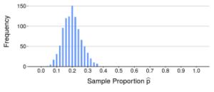
Question 5
Four graphs of 1,000 randomly generated sample proportions are shown. Match each plot with its corresponding values of [latex]n[/latex] and [latex]p[/latex].
- [latex]n= 20, p= 2[/latex]
- [latex]n= 20, p= 6[/latex]
- [latex]n= 50, p= 2[/latex]
- [latex]n= 50, p= 6[/latex]
Graph 1
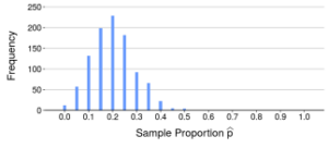
Graph 2
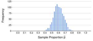
Graph 3
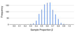
Graph 4