Preparing for the next class
In the next in-class activity, you will need to calculate the components of a confidence interval for a population proportion, including the point estimate, standard error, z critical values, and margin of error. You will also need to use these components to construct confidence intervals for proportions and represent them on number lines. To do this, you will need to understand the connection between sampling distributions, the Central Limit Theorem, and confidence intervals.
Question 1
Suppose we want to estimate the proportion of college students who have a high level of stress. In a previous homework assignment, we looked at a sample of 253 college students and found that 56 of them had high levels of stress.[1]
What proportion of students in the sample had a high level of stress?
Hint: To calculate the proportion, take the number of successes divided by the sample size.
Recall that in the previous activities, we assumed we knew the true population parameter, [latex]p[/latex], and looked at how close sample proportions were to this value. Often, we will not know the true population parameter, so we will need to estimate it. The sample proportion is used as a point estimate of the population proportion. A point estimate is a single value based on representative sample data that is a plausible estimate of the population parameter. In this case, we are talking about proportions, so the best estimate for the population proportion is the sample proportion. We refer to the point estimate for proportions as [latex]\hat{p}[/latex].
Question 2
Refer to Question 1 to answer the following questions.
- What do we want to estimate?
- The population proportion, [latex]p[/latex]
- The sample proportion, [latex]\hat{p}[/latex]
- What are we going to use to estimate the proportion of college students who have a high level of stress?
- The population proportion, [latex]p[/latex]
- The sample proportion, [latex]\hat{p}[/latex]
Question 3
Suppose we took another different sample of 253 college students. Would you expect the proportion of students with a high level of stress to be the same as in Question 1 or different from Question 1?
- The same
- Different
Recall from In-Class Activity 9.C:
Sampling Distribution of the Sample Proportion
When taking many, many random samples of size n from a population distribution with proportion [latex]p[/latex]:
The mean of the distribution of sample proportions is [latex]p[/latex].
The standard deviation of the distribution of sample proportions is[latex]\sqrt{\frac{p(1-p)}{n}}[/latex].
If [latex]np \geq 10[/latex] and [latex]n(1-p) \geq 10[/latex], then the Central Limit Theorem (CLT) states that the distribution of the sample proportions follows an approximate normal distribution with mean [latex]p[/latex] and standard deviation [latex]\sqrt{\frac{p(1-p)}{n}}[/latex].
Question 4
Is the sample size in Question 1 large enough to use the approximate distribution stated by the CLT?
Hint: Use the condition [latex]n\hat{p} \geq 10[/latex] and [latex]n(1−\hat{p}) \geq 10[/latex].
Question 5
What can we say about how close the sample proportion is to the population proportion?
- Approximately 68% of the sample proportions will fall within 2 standard deviations of the mean ([latex]p[/latex]).
- Approximately 95% of the sample proportions will fall within 2 standard deviations of the mean ([latex]p[/latex]).
- Approximately 99.7% of the sample proportions will fall within 2 standard deviations of the mean ([latex]p[/latex]).
Hint: Remember the Empirical Rule.
Recall that when the sample size is large enough, we can use [latex]\sqrt{\frac{\hat{p}(1-\hat{p})}{n}}[/latex] in place of[latex]\sqrt{\frac{p(1-p)}{n}}[/latex] . This is called the standard error, which is the estimated standard deviation of sample proportions. It is the measure of sample-to-sample variability. We will use the standard error to help us convey information about the accuracy of our point estimate!
Question 6
Calculate the estimated standard deviation for the sample proportion for the scenario in Question 1. Round your answer to 2 decimal places.
A confidence interval for a population proportion is a reasonable range of values where we expect the population proportion to fall within, with a chosen degree of confidence. We create confidence intervals because, as seen in previous in-class activities, sample proportions vary from sample to sample.
A sample proportion will most likely not be equal to the true population parameter. Thus, instead of simply using a single value (a point estimate) to estimate our parameter, we will use a range of values. Confidence intervals take sampling variability into account and convey information on estimate accuracy.
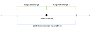
A confidence interval is calculated using the point estimate and the margin of error. The margin of error (E) is what determines the width of the interval. A confidence interval will have a width of twice the margin of error. The following is a visualization of a confidence interval.
The margin of error is calculated using the standard error and the z critical value for the confidence level. This means that the width of our interval is determined by how much our sample data varies and how confident we want to be in our method.
The confidence level, [latex]C[/latex], tells us how much confidence we have in the method used to construct the interval. It corresponds to the percentage of all intervals we would expect to contain the true population parameter.
For example, if we have a 95% confidence level and we took a very large number of different samples and created confidence intervals for each one, we would expect about 95% of them to contain the population parameter.
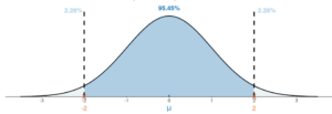
For proportions, each confidence level has a corresponding z critical value ([latex]z^{*}[/latex]). In Question 5, we applied the Empirical Rule, which indicates [latex]z^{*}= 2[/latex]and its negative counterpart, -2. As you can see below, the values of 2 separate the middle 95.45% from the most extreme 4.55% areas. Note that the most extreme area is split evenly in each tail.
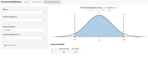
In practice, we are usually interested in 90%, 95%, and 99% confidence intervals. Below is the standard normal distribution displaying the z critical value, [latex]z^{*}[/latex], for a 95% confidence level. As you can see, 95% of the curve is shaded in and the remaining 5% of the curve is unshaded in the tails. The values that separate the middle 95% from the most extreme 5% are what we will use for our confidence interval.
The [latex]z^{*}[/latex] value is found using the DCMP Normal Distribution tool at https://dcmathpathways.shinyapps.io/NormalDist/.
- Select the Find Percentile/Quantile tab.
- The tool defaults to a standard normal distribution with mean [latex]\mu[/latex] = 0 and standard deviation [latex]\sigma[/latex]= 1.
- Select “Two-tailed” and enter 95 for “Central Probability,” since we want the middle 95%.
- The z critical value, [latex]z^{*}[/latex], is 1.96. Note the tool presents both the z critical value and its negative counterpart, -1.96.
Question 7
Use the Find Percentile/Quantile tab of the DCMP Normal Distribution tool to find the z critical value, [latex]z^{*}[/latex], for the most common confidence levels seen below.
| Confidence level, C | [latex]z^{*}[/latex] |
| 90% | |
| 95% | 1.96 |
| 99% |
Hint: Since you are looking at the standard normal distribution, you will keep the mean at 0 and the standard deviation at 1. You will need to use the two-tailed option.
Now that we have the standard error and z critical value, we can calculate the margin of error.
| Margin of error ([latex]E): E = z^{*} \bullet (standard~error)[/latex]
Let’s break down the margin of error. The margin of error is the width of the confidence interval and is comprised to two parts: Standard error: A measure of the sample-to-sample variability, [latex]\sqrt{\frac{\hat{p}(1-\hat{p})}{n}}[/latex]. [latex]z^{*}[/latex]: The z critical value; this is the point on the standard normal distribution such that the proportion of area under the curve between [latex]−z^{*}[/latex] and [latex]+z^{*}[/latex] is [latex]C[/latex], the confidence level. |
Question 8
Calculate the margin of error that would be used to create a 95% confidence interval for the population proportion of students who had a high level of stress. Round to 4 decimal places.
Hint: Use your answers from Questions 6 and 7. Remember the z critical value is positive.
Question 9
We can now create our confidence interval using the point estimate and the margin of error. We do this by adding and subtracting the margin of error to/from the point estimate. The point estimate will always be exactly in the center of our interval.
- Subtract the margin of error from the point estimate. This is the lower bound of the confidence interval.
- Add the margin of error to the point estimate. This is the upper bound of the confidence interval.
- Which of the following number lines correctly represents the point estimate, upper bound, and lower bound?
Question 10
Looking at the confidence interval represented on the following number line, answer the following questions.
![]()
- What is the value of the point estimate?
- What is the approximate margin of error?
- What is the approximate confidence interval? Write the confidence interval in the form (lower bound, upper bound), which is called interval notation form.
Hint: If the lower bound of the interval was at 0.8 and the upper bound of the interval was at 0.9, the confidence interval would be written as (0.8, 0.9).
| Confidence Intervals
In general, the end points of a confidence interval are: point estimate ± margin of error The confidence interval for a population proportion is: [latex]\hat{p} \pm z * x\sqrt{\frac{\hat{p^{*}}(1-\hat{p})}{n}}[/latex] |
- Onyper, S., Thacher, P., Gilbert, J., & Gradess, S. (2012). Class start times, sleep, and academic performance in college: A path analysis. Chronobiology International, 29(3): 318–335. ↵
