Preparing for the next class
In the next in-class activity, you will need to understand the limitations of the conclusions from the F-test in an ANOVA, identify the null and alternative hypotheses for all pair-wise comparisons, and use technology to perform a two-sample t-test. You will also need to identify the probability of type I errors and issues that arise with multiple comparisons and use adjusted confidence intervals to conduct all pair-wise tests and make conclusions about significant differences.
In In-Class Activities 14.A through14.C, we conducted a one-way ANOVA, which is a statistical test for comparing and making inferences about means associated with two or more groups.
In the next in-class activity, you will conduct a complete one-way ANOVA to make an overall comparison among the population means and further investigate the individual pair-wise differences in the means. You will also learn about the ramifications of conducting multiple statistical tests.
Question 1
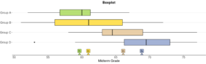
1) Suppose you are studying the efficacy of new statistics teaching methods. You randomly assign 20 students to each of the four different methods: A, B, C, and D. You test their knowledge on the midterm to compare the differences between the teaching methods. The results are shown in the following table and boxplots (continued on the next page). For this activity, you may assume the conditions for ANOVA are met.
| A | B | C | D |
| 59 | 67 | 62 | 69 |
| 54 | 66 | 74 | 62 |
| 60 | 51 | 62 | 70 |
| 57 | 68 | 64 | 73 |
| 58 | 65 | 77 | 53 |
| 52 | 54 | 59 | 73 |
| 67 | 57 | 58 | 75 |
| 61 | 55 | 64 | 64 |
| 54 | 59 | 68 | 67 |
| 56 | 66 | 65 | 73 |
| 62 | 70 | 66 | 69 |
| 60 | 56 | 64 | 69 |
| 56 | 56 | 73 | 72 |
| 61 | 53 | 65 | 73 |
| 67 | 56 | 67 | 73 |
| 65 | 72 | 72 | 59 |
| 61 | 64 | 63 | 77 |
| 61 | 64 | 72 | 62 |
| 60 | 63 | 63 | 77 |
| 62 | 57 | 64 | 67 |
Part A: What is the null hypothesis?
Part B: What is the alternative hypothesis?
The P-value for the test is presented in the following output:
ANOVA Table:
| Source | df | Sum of Squares | Mean Square | F Statistic | P-value |
| Group | 3 | 1122 | 374 | 12.46 | <0.0001 |
| Error | 76 | 2282 | 30.02 | ||
| Total | 79 | 3404 |
Part C: What should be the conclusion of the test?
Part D: Determine if this statement is true or false: I can use the conclusion of the ANOVA to identify which method is the best?
This leads us to the next logical question—which means are different? Once we have rejected the null hypothesis that all means are equal, we will want to perform multiple comparisons to identify the differences.
In In-Class Activity 13.C, we explored hypothesis tests that allowed us to compare means from two groups/populations. More specifically, we performed calculations to determine if there was evidence that the means associated with the populations were statistically different from one another.
Question 2
2) To compare all groups, we could perform six different two-sample t-tests in order to find the significant difference(s). Describe the six comparisons. Fill in the two group names in the missing blanks below.
- Group A vs. Group B
- Group A vs. Group ___
- Group A vs. Group D
- Group B vs. Group C
- Group B vs. Group ___
- Group C vs. Group D
Question 3
3) Suppose we want to compare Group A to Group B. Which of the following is the correct null hypothesis for this scenario?
- a) �0: �$ = �&
- b) �’: �$ = �& = �(
- c) �0: �$ = �& = �( = �)
- d) �0: �$ ≠ �&
Question 4
4) Which of the following is the appropriate alternative hypothesis for the scenario described in the previous question?
- a) �$: At least two of the group means are different.
- b) �$: At least three of the group means are different.
- c) �$: All of the group means are different.
- d) �$: �$ ≠ �&
Question 5
5) Use the DCMP Compare Two Population Means tool at https://dcmathpathways.shinyapps.io/2sample_mean/ to conduct a two-sample t-test to compare the midterm means of Group A and Group B.
Hint: Copy and paste from the table in Question 1.
Part A: What is the P-value of the test to the nearest hundredth?
Part B: What is the confidence interval for the difference �$ − �&?
Part C: At the 5% significance level, what can you conclude from your answers in Parts A and B? Do you prefer one of the two methods? Explain.
Question 6
6) Use the DCMP Compare Two Population Means tool to conduct a two-sample t-test to compare the midterm means of Group A and Group C.
Hint: Copy and paste from the table in Question 1.
Part A: What is the P-value of the test?
Part B: What is the confidence interval for the difference �$ − �(?
Part C: At the 5% significance level, what can you conclude from your answers in Parts A and B? Do you prefer one of the two methods? Explain.
We could continue and conduct all six different hypothesis tests/confidence intervals in order to determine exactly which means are different from one another.
Recall from In-Class Activity 11.E that sometimes, due to chance, the result of the hypothesis test does not align with reality. If we reject a correct null hypothesis, we have made a type I error. In summary, the probability of committing a type I error is equal to the significance level: [latex]P[/latex](type I error) = [latex]\alpha[/latex].
Question 7
7) If you conducted all six pair-wise comparisons using a two-sample t-test, what is the probability of committing a type I error in each of the following tests? Complete the following table.
| Comparison | Probability of Committing a Type I Error |
| Group A vs. Group B | 0.05 |
| Group A vs. Group C | |
| Group A vs. Group D | |
| Group B vs. Group C | |
| Group B vs. Group D | |
| Group C vs. Group D |
Question 8
8) If you conduct ALL six tests, do you think the probability of committing a type I error remains at 0.05? Explain.
Suppose we perform [latex]m[/latex] independent hypothesis tests. The probability of making a type I error (at least one false rejection) is:
[latex]1-(1-\alpha)^{m}[/latex]
In our example, we have six comparisons, so the probability of committing a type I error is:
[latex]1 − (1 − .05)^{6}= 0.265\;or\;26.5%[/latex]
This is likely too high and definitely not 0.05. To avoid this problem, we need a method to maintain an overall level of significance even when several tests are performed. We call this the family-wise error rate. The family-wise error rate is defined as the probability of rejecting at least one of the true null hypotheses.
One method for controlling for a family-wise error rate is the Tukey method for all pair wise comparisons (formally Tukey-Kramer method). This method adjusts the length of the confidence interval (to ensure an overall level of confidence) and the P-value (to ensure an overall significance level for all pair-wise comparisons).
Question 9
9) Compare the confidence intervals in Table A and Table B (next page). Table A presents the P-values and confidence intervals that are unadjusted for multiple comparisons. Table B presents the adjusted confidence intervals using the Tukey method.
Table A: Unadjusted for multiple comparisons*
| Comparison | Estimated Difference In Means | Standard Error | t Statistic | P-value | Lower Bound | Upper Bound |
| Group A vs. Group B | -1.30 | 1.73 | -0.75 | 0.45 | -4.75 | 2.15 |
| Group A vs. Group C | -6.45 | 1.73 | -3.72 | 0.00 | -9.90 | -3.00 |
| Group A vs. Group D | -9.20 | 1.73 | -5.31 | 0.00 | -12.65 | -5.75 |
| Group B vs. Group C | -5.15 | 1.73 | -2.97 | 0.00 | -8.60 | -1.70 |
| Group B vs. Group D | -7.90 | 1.73 | -4.56 | 0.00 | -11.35 | -4.45 |
| Group C vs Group D | -2.75 | 1.73 | -1.59 | 0.11 | -6.20 | 0.70 |
*Note: These P-values and confidence intervals are slightly different than those derived from conducting separate two-sample t-tests.
Table B: Tukey method used to adjust for multiple comparisons
| Comparison | Estimated Difference in Means | Standard Error | t Statistic | Multiplicity Adjusted P-value | Lower Bound | Upper Bound |
| Group A vs. Group B | -1.30 | 1.73 | -0.75 | 0.88 | -5.85 | 3.25 |
| Group A vs. Group C | -6.45 | 1.73 | -3.72 | 0.00 | -11.00 | -1.90 |
| Group A vs. Group D | -9.20 | 1.73 | -5.31 | 0.00 | -13.75 | -4.65 |
| Group B vs. Group C | -5.15 | 1.73 | -2.97 | 0.02 | -9.70 | -0.60 |
| Group B vs. Group D | -7.90 | 1.73 | -4.56 | 0.00 | -12.45 | -3.35 |
| Group C vs. Group D | -2.75 | 1.73 | -1.59 | 0.39 | -7.30 | 1.80 |
Part A: What are the unadjusted confidence interval and P-value that compare Group B and Group C?
Hint: Look at upper and lower bounds.
Part B: What are the Tukey method adjusted confidence interval and P-value that compare Group B and Group C?
Part C: Which interval is shorter in length?
Part D: Examine the adjusted confidence interval to determine whether the confidence interval includes the value of 0 (no difference in means). Is the mean midterm score of Group B significantly different from the mean midterm score of Group C? Explain.
Part E: What can you conclude from the confidence interval? Which teaching method would you prefer between the methods for Group B and Group C?
Hint: In this case, the adjusted confidence interval is for the difference �& − �(.
Note that the difference between the methods for Group C and Group B [latex]\mu_{C}−\mu_{B}[/latex] is not considered because it would provide the same information. Similarly, [latex]\mu_{C}−\mu_{A}[/latex] etc. are not needed.
Question 10
10) Use the adjusted confidence intervals to complete the following table. Add the comparisons to the appropriate column. The first two comparisons are done for you.
| Significantly Different Mean Midterm Grades | NOT Significantly Different Mean Midterm Grades |
| Group A vs. Group C | Group A vs. Group B |
