
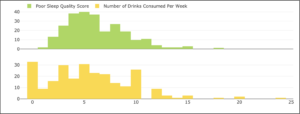
| Poor Sleep Quality Score | Alcoholic Drinks Per Week | |||
| Mean | Median | Mean | Median | |
| Owl | ||||
| Lark | ||||
| Neither |
| Mean | Median | |
| Owl | 4.24 | 2 |
| Lark | 1.57 | 1 |
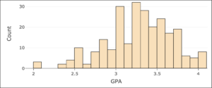
| Class | Mean | Median |
| Freshman (Year 1) | ||
| Sophomore (Year 2) | ||
| Junior
(Year 3) |
||
| Senior
(Year 4) |
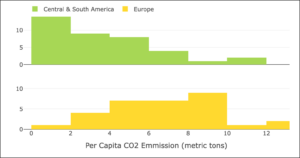
| Group | Mean | Median |
| Central and South America | ||
| Europe |
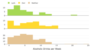
| Group | Mean | Median |
| Owl | ||
| Lark | ||
| Neither |
| Skill or Concept: I can . . . | Questions to check your understanding | Rating from 1 to 5 |
| Calculate the mean and median of a dataset by hand, as well as with technology. | 1, 2 | |
| Calculate the mean and median for multiple groups using technology. | 4 | |
| Estimate the mean and median by looking at the data presented in a histogram. | 3, 5 |
Glossary
- mean
- the arithmetic mean of a list of numbers, commonly called the “average”.
- median
- the “middlemost” number.
