| State | Average Daily Screen Time
(in minutes) |
State | Average Daily Screen Time (in minutes) | |
| Alabama | 170 | Montana | 154 | |
| Alaska | 134 | Nebraska | 182 | |
| Arizona | 276 | Nevada | 262 | |
| Arkansas | 145 | New Hampshire | 135 | |
| California | 204 | New Jersey | 182 | |
| Colorado | 166 | New Mexico | 177 | |
| Connecticut | 262 | New York | 206 | |
| Delaware | 166 | North Carolina | 205 | |
| Florida | 213 | North Dakota | 192 | |
| Georgia | 198 | Ohio | 231 | |
| Hawaii | 133 | Oklahoma | 131 | |
| Idaho | 161 | Oregon | 132 | |
| Illinois | 220 | Pennsylvania | 213 | |
| Indiana | 220 | Rhode Island | 165 | |
| Iowa | 163 | South Carolina | 155 | |
| Kansas | 146 | South Dakota | 154 | |
| Kentucky | 149 | Tennessee | 196 | |
| Louisiana | 144 | Texas | 186 | |
| Maine | 165 | Utah | 155 | |
| Maryland | 199 | Vermont | 124 | |
| Massachusetts | 195 | Virginia | 179 | |
| Michigan | 188 | Washington | 173 | |
| Minnesota | 140 | West Virginia | 150 | |
| Mississippi | 146 | Wisconsin | 211 | |
| Missouri | 211 | Wyoming | 134 |
| Symbol | Description | |
| difference between the population means | ||
| population mean of Group 1 | ||
| sample standard deviation of Group 1 | ||
| sample size of Group 1 | ||
| sample mean of Group 2 | ||
| difference between the sample means | ||
| sample mean of Group 1 | ||
| population mean of Group 2 | ||
| sample size of Group 2 | ||
| sample standard deviation of Group 2 |
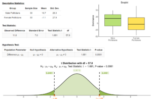
| Group 1:
smoke_now = Yes Mothers who smoked during pregnancy |
Group 2:
smoke_now = No Mothers who did not smoke during pregnancy |
|
| Sample Mean | 114 | = 123 |
| Sample Standard Deviation | = 18.2 | = 17.3 |
| Sample Size | = 480 | = 733 |
| Group 1: Female Professors | Group 2: Male Professors | |
| Sample Size | 40 | 53 |
| Sample Mean Course Evaluation Score | 3.79 | 4.01 |
| Sample Standard Deviation | 0.51 | 0.53 |
| Community College Transfer (Group 1) | No Transfer (Group 2) | |
| Sample Size | 267 | 1176 |
| Sample Mean Time to Graduate, in Years | 5.37 | 4.45 |
| Sample Standard Deviation Time to Graduate, in Years | 1.175 | 1.001 |
| gestation | smoke | smoke_now | age | wt |
| 284 | never | No | 27 | 120 |
| 282 | never | No | 33 | 113 |
| 279 | now | Yes | 28 | 128 |
| 282 | now | Yes | 23 | 108 |
| 286 | until current pregnancy | No | 25 | 136 |
| 244 | never | No | 33 | 138 |
| 245 | never | No | 23 | 132 |
| 289 | never | No | 25 | 120 |
| 299 | now | Yes | 30 | 143 |
| 351 | once did, not now | No | 27 | 140 |
| Group 1:
smoke_now = Yes Mothers who smoked during pregnancy |
Group 2:
smoke_now = No Mothers who did not smoke during pregnancy |
|
| Sample Mean |
= ____ |
|
| Sample Standard Deviation |
= ______
|
= ______
|
|
Sample Size |
= ______
|
= _____
|
| Skill or Concept: I can . . . | Questions to check your understanding | Rating from 1 to 5 |
| Use appropriate notation to represent the sample mean, sample standard deviation, and sample size for multiple groups. | 1, 2 | |
| Write an expression that represents the difference between two sample means and the difference between two population means. | 3 | |
| Verify that conditions are met for a two-sample t-test for independent samples. | 4 | |
| Calculate the standard error for a sampling distribution and interpret its meaning. | 5 | |
| Use descriptive statistics to describe the difference between two sample means and interpret its meaning. | 6, 7 |
Glossary
- two-sample t-test
- a hypothesis test for comparing two population means.
