Preparing for the next class
In the next in-class activity, you will need to make connections between values presented in an ANOVA table and describe the shape of the F Distribution. You will also need to understand how the P-value is represented by an area under an F Distribution curve and describe how the F-statistic is used in hypothesis testing for a one-way ANOVA. Finally, you will need to use the P-value to reach a conclusion.
Suppose a researcher wants to investigate the effect of the amount of fertilizer on the height of a common houseplant. More specifically, the researcher is interested in determining if there is a difference in the mean height of plants between those receiving one of following three different fertilizer levels: high, medium, and low.
The following data are the simulated results of this controlled experiment. (Note that this small dataset is used introduce the concept and make calculations easier. When conducting an ANOVA, larger sample sizes are usually needed to meet assumptions.)
| Fertilizer Level | Height of Plant (inches) |
| Low | 23.2, 20.9, 21.5, 25.3 |
| Medium | 24.6, 27.7, 22.5, 30.1 |
| High | 29.2, 30.2, 31.1, 33.6 |
As we saw in the previous in-class activity, conducting a one-way ANOVA involves comparing the variation within each of the groups to the variation between each of the groups. When the variation between each of the groups is significantly larger than the variation within each of the groups, we might conclude that there is a statistically significant difference among the means.
In an ANOVA table, the calculation illustrating the total variation within the groups of interest is known as the error sum of squares (SSError). The calculation illustrating the total variation between the groups is known as the group sum of squares (SSGroup).
Two other essential columns found in an ANOVA table are the degrees of freedom (df) and the mean square.
The following table illustrates how these values are calculated for each of the given sources: Group or Error (i.e., between and within).
When calculating these values, it is important to know that [latex]k[/latex] represents the number of groups being considered and [latex]N[/latex] represents the total number of data values among all groups.
| Source | Degrees of Freedom (df) | Sum of Squares | Mean Square | F-Statistic |
| Group | [latex]k-1[/latex]
(The number of groups minus 1) |
SSGroup | SSGroup
[latex]k-1[/latex] |
MSGroup
MSError |
| Error | [latex]N-k[/latex]
(The total number of data points minus the number of groups) |
SSError | SSError
[latex]N-k[/latex] |
|
| Total | [latex]N-1[/latex]
(The total number of data points minus 1) |
SSGroup + SSError |
Question 1
Part A: In the fertilizer and plant height scenario, what is the value for � (i.e., the number of groups)?
Part B: In the fertilizer and plant height scenario, what is the value for � (i.e., the total number of data values in the experiment)?
Part C: Given your previous responses, complete the Degrees of Freedom column for the fertilizer and plant height scenario in the following table.
| Source | Degrees of
Freedom (df) |
| Group | k − 1 = |
| Error | N − k = |
| Total | N − 1 = |
When performing a formal hypothesis test for a one-way ANOVA, the mean square values are used to calculate the value of our test statistic; thus, they impact the P-value we get.
As noted in the previous table, the mean square for error and mean square for group are calculated by taking each of the sum of square values and dividing them by the degrees of freedom associated with the respective source (i.e., Group or Error).
[latex]Mean\;Square\;for\;Error\;(MSError)=\frac{Error\;sum\;of\;squares}{degrees\;of\;freedom\;(Error)}=\frac{SSE}{N-k}[/latex]
[latex]Mean\;Square\;for\;Group\;(MSGroup)=\frac{Group\;sum\;of\;squares}{degrees\;of\;freedom\;(Group)}=\frac{SSG}{k-1}[/latex]
Question 2
2) We are given the sum of squares and degrees of freedom for the fertilizer and plant height scenario. Use these values to calculate the mean square for error and mean square for group. Enter the values in the following table.
| Source | Degrees of
Freedom (df) |
Sum of Squares | Mean Square |
| Group | 2 | 55.9134 | |
| Error | 9 | 140.0108 | |
| Total | 11 | 195.9242 |
Question 3
3) The test statistic that we use to complete the appropriate hypothesis test for a one way ANOVA is calculated with the ratio below:
F-Statistic = MSGroup
MSError = Variation BETWEEN groups
Variation WITHIN groups
Use the MSGroup and MSError values you calculated to find the F-statistic for this situation:
F-Statistic = MSGroup
MSError = Variation BETWEEN groups
Variation WITHIN groups =
Question 4
4) Recall from previous in-class activities that hypothesis testing for two means is based on the t Distribution, and we calculate the test statistic, t. ANOVA is based on the F Distribution, so we will be calculating the F-statistic.
Go to the DCMP F Distribution tool at https://dcmathpathways.shinyapps.io/FDist/.
Using the data analysis tool, graph the F Distribution from the example by entering the degrees of freedom from Question 1, Part C or by selecting varying values.
Part A: The F Distribution is:
a) Skewed left
b) Symmetric
c) Skewed right
Part B: The t Distribution is symmetric, centered at the mean 0. Thus, when conducting a t-test, we have positive t-values and negative t-values. Adjust the numerator and denominator degrees of freedom in the F Distribution tool. What do you notice about the values in the F Distribution (the values on the horizontal axis)?
a) The F values are always negative.
b) The F values are always positive.
c) The F values can be negative or positive.
As we just saw, the F-statistic is the ratio of the variation between groups (MSGroup) to the variation within groups (MSError). Larger values of the F-statistic (greater than 1) would imply that the variation between groups is larger than the variation within groups.
Question 5
5) As the variation between groups gets significantly larger than the variation within groups, we will get:
- a) A larger F-statistic that corresponds to a greater P-value and less evidence to support the null hypothesis
- b) A larger F-statistic that corresponds to a smaller P-value and more evidence to support the alternative hypothesis
- c) A P-value that does not change as the F-statistic changes
When there is a greater difference among the group means, the F-statistic will be larger; when there is a smaller difference among the group means, the F-statistic will be smaller.
Question 6
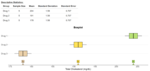
6) Which of the following plots will likely have the largest F-statistic? Explain. Note that the means for each group are exactly the same in Plot A and Plot B.
Plot A
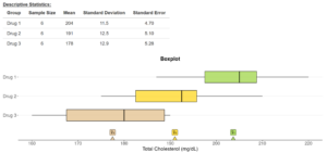
Plot B
Remember that in hypothesis testing, the P-value is our statistical evidence to support our conclusions. When the P-value is less than our significance level, α, we reject the null hypothesis and have sufficient evidence to support the alternative hypothesis. Otherwise, we fail to reject the null hypothesis and do not have sufficient evidence to support the alternative hypothesis.
Question 7
7) Suppose we ran an ANOVA at the alpha (α) = 0.05 significance level to answer the following question: “Is there a difference in the mean hours of exercise per week among people in the U.S. regions of the Northeast, South, West, and Midwest?”
Part A: If the test resulted in a P-value of 0.0245, what should you do? a) Reject the null hypothesis.
- b) Fail to reject the null hypothesis.
- c) Accept the null hypothesis.
Part B: Based on your answer to Part A, what would be your conclusion?
- a) There is convincing evidence to suggest that there is a difference in the mean hours of exercise between at least two regions.
- b) There is convincing evidence to suggest that there is a difference in the mean hours of exercise between all four regions.
- c) There is not convincing evidence to suggest that there is a difference in the mean hours of exercise between the four regions.
Question 8
8) Suppose we ran an ANOVA at the alpha (α) = 0.05 significance level for the following question: “Is there is a difference in the mean reduction of blood pressure for the following three different techniques: diet, exercise, and medication.”
Part A: If the test resulted in a P-value of 0.3214, what should you do? a) Reject the null hypothesis.
- b) Fail to reject the null hypothesis.
- c) Accept the null hypothesis.
Part B: Based on your answer to Part A, what would be your conclusion?
- a) There is convincing evidence that there is a difference in the mean blood pressure reduction between at least two techniques.
- b) There is convincing evidence that there is a difference in the mean blood pressure reduction between all three techniques.
- c) There is not convincing evidence that there is a difference in the mean blood pressure reduction between the three techniques.
