| 425 | 469 | 300 | 490 | 415 | 285 | 507 | 336 | 503 | 442 |
| 307 | 317 | 251 | 397 | 294 | 263 | 406 | 262 | 391 | 356 |
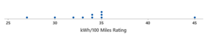
| Observation | Car model | kWh/100 miles |
| 1 | Porsche Taycan 4S Cross Turismo | 45 |
| 2 | Volkswagen ID.4 Pro S | 35 |
| 3 | Hyundai Kona Electric | 27 |
| 4 | Ford Mustang Mach-E RWD | 34 |
| 5 | Tesla Model S Performance | 35 |
| 6 | Tesla Model X Performance | 35 |
| 7 | Nissan Leaf SV/SL | 32 |
| 8 | Tesla Model S Plaid | 33 |
| 9 | Volkswagen ID.4 Pro | 34 |
| 10 | BMW i3s | 30 |
| Random number | kWh/100 miles |
| Random number | kWh/100 miles |
| Skill or Concept: I can . . . | Questions to check your understanding | Rating from 1 to 5 |
| Understand how fuel efficiency is measured for electric cars. | 1 | |
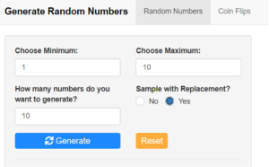
| Use technology to generate random numbers. | 2 | |
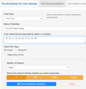
| Select a bootstrap sample and calculate its mean. | 2 |

![Some tables and graphs. The first table is titled “Summary Statistics For Bootstrap Distribution.” The columns are “Bootstrap Samples,” “Statistic,” “Unique Values,” “Mean,” “Standard Deviation,” “Min,” “Q1,” “Median,” “Q3,” and “Max.” The values are 1,000, Mean, 605, 417, 24.4, 346, 400, 419, 434, and 481. Beneath this table is a graph titled “Bootstrap Sampling Distribution” and labeled “Sample Mean x bar” on the x-axis and “Frequency” on the y-axis. The graph has a peak at approximately 420. There is a label reading “2.5th Percentile” at approximately 365, another label reading “Observed Mean” at approximately 420, and another label reading “97.5th Percentile” at approximately 465. Beneath this graph is another graph titled “95% Bootstrap Confidence Interval” and labeled “Population Mean (C02 Emission Rating)” on the x-axis. It has a point at approximately 415 with a range labeled as “[367, 463].” Beneath this is another table, this one titled “Bootstrap Percentile Confidence Interval.” It has columns “Population Parameter,” “Point Estimate,” “Lower Bound,” “Upper Bound,” and “Confidence Level.” The values are “Mean,” 417, 367, 463, and 95%.](https://s3-us-west-2.amazonaws.com/courses-images/wp-content/uploads/sites/5738/2022/01/27022934/Picture1331-300x135.png)
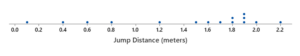
| 0.1 | 0.4 | 0.6 | 0.8 | 1.3 | 1.5 | 1.6 | 1.7 |
| 1.8 | 1.8 | 1.9 | 1.9 | 1.9 | 2.0 | 2.2 |
| 0.1 | 0.4 | 0.6 | 0.8 | 1.3 | 1.5 | 1.6 | 1.7 |
| 1.8 | 1.8 | 1.9 | 1.9 | 1.9 | 2.0 | 2.2 |
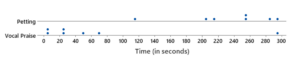
| Petting | 114 | 203 | 217 | 254 | 256 | 284 | 296 |
| Vocal praise | 4 | 7 | 24 | 25 | 48 | 71 | 294 |
| 0.1 | 0.4 | 0.6 | 0.8 | 1.3 | 1.5 | 1.6 | 1.7 |
| 1.8 | 1.8 | 1.9 | 1.9 | 1.9 | 2.0 | 2.2 |
| Petting | 114 | 203 | 217 | 254 | 256 | 284 | 296 |
| Vocal praise | 4 | 7 | 24 | 25 | 48 | 71 | 294 |
| Skill or Concept: I can . . . | Questions to check your understanding | Rating from 1 to 5 |
| Create a bootstrap confidence interval for a population median. | 1 | |
| Determine when it is appropriate to use a two-sample t confidence interval to estimate a difference in means. | 2 |
Descriptive Statistics:
| Group | Sample Size | Mean | Std. Dev. | Min | Q1 | Median | Q3 | Max |
| Petting | 7 | 232.0 | 61.7 | 114 | 210.0 | 254 | 270 | 296 |
| Vocal Praise | 7 | 67.6 | 102.5 | 4 | 15.5 | 25 | 59.5 | 294 |
Glossary 18A
- sampling without replacement
- sampling where once an individual from the population is selected for the sample and data are recorded for that individual, they are not considered again when making additional selections from the population for that sample.
- sampling with replacement
- sampling where after an individual is selected for the sample and data are recorded for that individual, they are “replaced” (put back into the population) before the next selection is made.
- bootstrap sample
- a sample that is selected from the values in the original sample.
