18B InClass

Every year, bullfrogs compete in a jumping contest at the Calaveras County Jumping Frog Jubilee (a contest inspired by a short story by Mark Twain). One year, researchers recorded the jump distances of frogs entered in the contest.^[1]

Question 1

1) The following are the jump distances (in meters) for a sample of 15 bullfrogs.

0.1	0.4	0.6	0.8	1.3	1.5	1.6	1.7
1.8	1.8	1.9	1.9	1.9	2.0	2.2

A dotplot of the sample jump distances is shown here.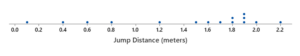 A dotplot titled “Jump Distance (meters).” There is a dot at 0.1, another at 0.4, another at 0.6, another at 0.8, another at 1.2, another at 1.5, another at 1.6, another at 1.7, two at 1.8, three at 1.9, another one at 2.0, and one more at 2.2. If we were interested in estimating the population mean jump distance (the mean jump distance for all frogs entered in the competition), it would not be appropriate to use a one-sample t confidence interval because the sample size is not greater than 30 and, because the data distribution is skewed, it is not reasonable to think that the population jump distance distribution is approximately normal.

Part A: What would be a more appropriate way to create a confidence interval for the population mean?

When a greater number of bootstrap samples are used to create the bootstrap distribution, there is less variability in the confidence intervals produced by different simulations.Youwill be able to:Use technology to construct a bootstrap confidence interval for a population median.Use technology to construct a bootstrap confidence interval for a difference in two population means.Interpret bootstrap confidence intervals.

Part B: Compute thevalues of the mean and the median for this dataset. Do you thinkthe mean or the medianis a better choice for describing a typical value for this dataset?

Part C: Up to this point in the course, we have not seen how to construct confidence intervals for population parameters other than means and proportions. But in this context, we really would like to use sample data to construct a confidence interval for thepopulation medianrather than the mean. Do you have any ideas on what we might do? The followingare the steps for constructinga bootstrap confidence interval for a population median:

1. Create a bootstrap sample by selecting a sample with replacement from theoriginalsample.

2. Calculate the sample medianfor the bootstrap sample.

3. Repeat Steps 1 and 2 a large number of times.

4. Create a bootstrap distribution of the bootstrap sample medians and thendetermine the end points of the confidence interval by using appropriatepercentiles of the bootstrap distribution. To calculate a bootstrap confidence interval, we can use the app athttps://istats.shinyapps.io/Boot1samp/.•For the “Enter Data” option,choose “Your Own.”•For “Name of Variable,” type “Jump Distance.”•Type the values from the sample into the “Enter Observations” box. Separate the data values by spaces or commas. The values for the sample are: 0.1, 0.4, 0.6, 1.2, 0.8, 1.5, 1.6, 1.7, 1.8, 1.8, 1.9, 1.9, 1.9, 2.0, and 2.2.•For the “Statistic of Interest” option, select “Median.”•Click on “1,000”for “Selecthow many bootstrap samples you want to generate,”and then click on “Draw Bootstrap Sample(s).”

Question 2

2) When you have completed thesesteps, you should see the bootstrap distribution in the lower part of the right-hand side of the display.

Part A: Is the bootstrap distribution symmetric or skewed?Once the bootstrap distribution has been prepared, it is possible to calculate a bootstrap confidence interval. At the very top of the display, click on the Get Confidence Intervaltab. Check to make sure that the confidence level is set to 95%. The corresponding bootstrap confidence interval is on the right-handside of the display.

Part B: What did you get for the 95% confidence intervalfor the population median?

Part C: The median for the original sample was 1.7 meters. Is the confidence interval symmetric around the sample median of 1.7?Does this surprise you? (Hint: Is 1.7 at the center of the confidence interval?)

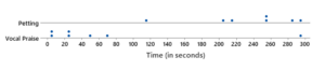
Questions 3–5 revisit the dog interaction times data from the preview assignment. Researchers measured the amount of time a dog spent interacting with its owner during a five-minute period while the owner was offering petting for a sample of seven adult dogs. They also measured the amount of time a dog spent interacting with its owner during a five-minute period while the owner was offering vocal praise for a sample of seven adult dogs. We will assume that each of the two samples of dogs are representative of the population of all adult dogs and that the samples were independently selected.The following are the data for the two samples and the corresponding dotplots (continued on the next page). Time spent was measured in seconds.

Petting	114	203	217	254	256	284	296
Vocal praise	4	7	24	25	48	71	294

Two side-by-side dot plots labeled “Time (in seconds)” on the x-axis. The first plot is labeled “Petting” and has a point at approximately 115, another at approximately 205, another at approximately 215, two at approximately 255, another at approximately 285, and another at approximately 295. The second plot is labeled “Vocal Praise” and has two dots at approximately 5, two at approximately 25, one at approximately 50, another at approximately 70, and another at approximately 295.

Question 3

3) One possibility might be to consider using the two-sample t confidence intervalto estimate the difference in population means. In the preview assignment, you decided that this wasn’t reasonable. Whyis it not reasonable?

If a two-sample t confidence interval is not appropriate, what can do we instead? It probably won’t surprise you that we could use a bootstrap confidence interval! When we have two samples and want to estimate a difference in population means, we focus on the difference in the two sample means. If we had chosen different samples of the same size, we would have seen different sample means and a different value for the difference in sample means. What differences in the sample means could have arisen? Bootstrapping constructs more possible differences in sample means by generating a bootstrap sample from each of the original samples and calculating the difference in the bootstrap sample means. If this process is repeated a large number of times to form a bootstrap distribution, we can use that distribution to construct a 95% bootstrap percentile confidence interval by identifying the 2.5% and the 97.5% percentiles from the bootstrap sampling distribution. The software we use for constructing a bootstrap percentile confidence interval for a difference in means is the app athttps://istats.shinyapps.io/Boot2samp/. Go to the app and then:

•For the “Enter Data” option, select “From Textbook.”

•For “Dataset,” select “Petting vs. Vocal Praise.”

•For the “Statistic of Interest” option, select “Difference Between Means.”

Question 4

4) The right-hand side of the screen shows the following table of descriptive statistics for the original dog interaction time samples.

Descriptive Statistics:

Group	Sample Size	Mean	Std. Dev.	Min	Q1	Median	Q3	Max
Petting	7	232.0	61.7	114	210.0	254	270	296
Vocal Praise	7	67.6	102.5	4	15.5	25	59.5	294

Part A: What is the sample mean interaction time for the petting sample, based on thesedata?

Part B: What is the sample mean interaction time for the vocal praise sample, based on thesedata?

Part C: What is the difference in sample means (petting minus vocal praise),based on thesedata? Now you are ready to create the bootstrap distribution for the difference in sample means. Under the left-hand side of the screen prompt “Select how many bootstrap samples you want to generate,” click “1,000.” Under “Options,” check the box labeled “Summary Statistics of Bootstrap Distb.” Finally, press the button that says “Draw Bootstrap Sample(s).” The app willsample the pettingdata with replacement and separately sample the original vocal praisedata with replacementand then calculate each group’s mean and the differencein the means.

Question 5

5) This is repeated 1,000 times,and the 1,000 differences in sample means form a bootstrap distribution that appears on the right-handside of the screen.

Part A: On the right-hand side (under the dotplots)is a histogram of the differencesin sample means resulting from the bootstrap samples. Describe the distribution of the bootstrap differencesin sample means.

Part B: To find the bootstrap confidence interval for the difference in population means, click on the Find Confidence Intervaltab at the top of the screen.What is a 95% confidence interval for the difference in mean time spent interacting with owners for dogs that are offered petting and dogs that are offered vocal praise?

Part C: We can interpret thebootstrap confidence interval just like we have interpreted the two-sample t confidence interval for a difference inmeans. Writea sentence that interprets the bootstrap confidence interval for the difference in population means.

Question 6

6) In the examples considered so far, we have constructed bootstrap distributions using 1,000 bootstrap samples. This probably seems like a lot! In this question, we will consider why we need to use so many.

Part A: Using the dog interaction time data, go back and generate threedifferent 95% confidence intervals using only 100 bootstrap samples to form the bootstrap distributioneach time. Don’t forget to click the “Reset” button each time. What are the three confidence intervals you obtained?

Part B: Why aren’t the three 95% confidence intervals the same?

Part C: Using the dog interaction time data, go back and generate threedifferent 95% confidence intervals using 1,000 bootstrap samples to form the bootstrap distribution. Don’t forget to click the “Reset” button each time.What are the three confidence intervals you obtained?

Part D: What do you notice about the variability in the intervals produced by differentbootstrap simulationswhenthe intervals are based on only 100 bootstrap samples compared to when they are basedon 1,000 bootstrap intervals?

Part E: Would you recommend using 1,000 bootstrap samples or 100 bootstrap samples to construct a confidence interval? Explain.