You and your family are playing a board game that has a spinner with 6 equally-sized sections of different colors: red, orange, yellow, green, blue, and purple. In the first 5 spins, the spinner lands on the purple section 4 times.

Credit: iStock/SolStock
Question 1
Would this outcome make you suspicious that there is something wrong with the spinner?
Question 2
Suppose the spinner is fair, meaning that the arrow is equally likely to land on each of the 6 sections. You spin it 5 times and count how many times it lands on purple. Let [latex]X =[/latex] the number of times the spinner lands on purple. What are the possible values for [latex]X[/latex]?
This variable [latex]X[/latex] is classified as a discrete variable because it takes a fixed set of possible numerical values and it is not possible to get any value in between.
A probability distribution includes all possible values of a random variable and the probabilities associated with those values. Probability distributions can be constructed empirically using simulation.
Question 3
We want to model how often a fair spinner would land on purple, but we don’t have any spinners. How else could we model this situation?
Question 4
Everyone in the class will simulate 5 “spins” and record how many times they get “purple.” Then they will add their values to the class dotplot.
- Which value do you expect to occur most often?
- What shape do you expect the graph to have: roughly symmetric or skewed?
- Do you think anyone in the class will get the color purple 5 times? If not, what do you think the largest number will be?
Question 5
Sketch the class dotplot.
Question 6
Let [latex]X =[/latex] the number of times the spinner lands on purple. Based on the results of the simulation, estimate the probability of each possible value of this random variable. Record your answers in the following table.
| [latex]X =[/latex] Number of Purples | Probability |
| 0 | |
| 1 | |
| 2 | |
| 3 | |
| 4 | |
| 5 |
Question 7
What could we do to obtain more accurate empirical estimates of the probability?
Probability distributions can also be constructed theoretically using probability rules. The graph and table below show the theoretical probability of each outcome. (In In-Class Activity 8.C, you will learn to calculate these values.)
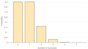
Note: Landing on purple is considered a “success” in this chance experiment.
| [latex]X =[/latex] Number of Purples | Probability |
| 0 | 0.4019 |
| 1 | 0.4019 |
| 2 | 0.1608 |
| 3 | 0.0322 |
| 4 | 0.0032 |
| 5 | 0.0001 |
Question 8
What is the sum of all the probabilities in the probability distribution? Round to 3 decimal places.
Question 9
Calculate the probability of landing on purple 4 or more times out of 5 spins if the spinner was really fair.
Question 10
If you were playing a board game and you landed on purple 4 or more times out of 5 spins, would you be convinced that something was wrong with the spinner?
Question 11
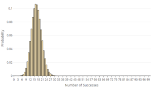
It’s difficult to judge whether or not the spinner is fair based on only 5 spins. With the Law of Large Numbers in mind, you decide to spin the spinner 100 times. How many times would the spinner have to land on purple for you to be convinced that the spinner was biased toward purple? Justify your answer based on the following probability distribution, which shows the outcomes we’d expect if the spinner was fair. Note: Landing on purple is considered a “success” in this chance experiment.
So far, we have been using a discrete probability distribution that gives the probabilities for a fixed set of values. The spinner can land on purple 2 or 3 times, but 2.5 is impossible. It is not in the set of possible values.
However, some variables are continuous, which means the range of values includes an infinite number of possible values. Consider a person’s height. Although we often measure heights to the nearest inch, a person does not grow in one inch spurts but instead moves through the range of heights via immeasurably small increments. It is not possible to count all the possible heights that a person can be because even between 64 inches and 65 inches, there are infinitely many possible heights.
When we are using a discrete probability distribution, we calculate the probability for a range of values by adding up the probability of each outcome in the range. However, when we are using a continuous probability distribution, probabilities are represented as the area under a density curve. The total area under the curve is equal to 1.
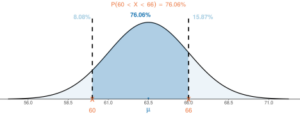
For example, suppose the following graph shows the distribution of heights (in inches) for women in a particular country. To find the probability that a randomly selected woman is between 60 and 66 inches tall, we would shade the area under the curve between these two values.
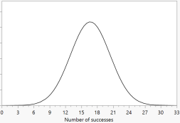
In some situations, we may use a continuous probability distribution as an approximation even when the variable is technically discrete. Let’s revisit the example of spinning a fair spinner 100 times, and let [latex]X =[/latex] the number of times the spinner lands on purple. The following graph shows a continuous probability distribution used as an approximation to the discrete distribution of [latex]X[/latex].
Question 12
Mark the following graph to show the probability of landing on purple 20 or more times in 100 spins.
Question 13
Is it unlikely for a fair spinner to land on purple 20 or more times out of 100? Explain.
