Each month, the U.S. Bureau of Labor Statistics releases a report on the employment situation in the United States. Included in the report is an estimate of the nationwide unemployment rate—the number of unemployed people as a percentage of the labor force (defined as the total number of employed individuals plus unemployed individuals who are actively looking for work).[1]
For example, at the start of the COVID-19 pandemic in the United States, the unemployment rate jumped from 3.5% in February 2020 to 14.8% in April 2020.[2]

Question 1
If you would have taken a random sample of 1,000 individuals from the U.S. labor force in April 2020 and calculated the percentage of those individuals who were unemployed, do you think you would have gotten 14.8%? Explain.
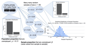
In this in-class activity, we will use the DCMP Sampling Distribution of the Sample Proportion tool to explore sampling variability of sample proportions. Our population will be the U.S. labor force, and we will assume that the true unemployment rate (the proportion of the U.S. labor force that is unemployed) is 0.15. In the tool:
- Set the Population Proportion ([latex]p[/latex]) to 0.15.
- Set the Sample Size ([latex]n[/latex]) to 50.
Question 2
Use the tool to select one random sample of size 50 from this population by clicking “1” and then “Draw Sample(s).” A bar graph of your randomly generated sample will be displayed directly under the graph of the population distribution.
- What is the value of your sample proportion?
- What is the appropriate statistical notation for this value?
Question 3
Select four more random samples of size 50 and fill in the following table with your five randomly generated sample proportions.
| Sample | Sample
Proportion |
| 1 | |
| 2 | |
| 3 | |
| 4 | |
| 5 |
Question 4
Explain why the values of sample proportions vary from sample to sample.
In order to get a sense of the pattern of variation in sample proportions, we need to generate more than five samples. The distribution showing how sample proportions vary from sample to sample is called a sampling distribution of the sample proportion.
In statistics, we often talk about “distributions,” and a “sampling distribution” is just a distribution of sample statistics as they vary from sample to sample. An illustration of the distinction between the population distribution of the variable (whether or not an individual is unemployed), a single sample distribution of the variable (still, whether or not an individual is unemployed), and the sampling distribution of sample
proportions (not the individual values of the variable but a statistic calculated from the values in a sample) are shown below.
Question 5
Use the DCMP Sampling Distribution of the Sample Proportion tool to generate 1,000 more sample proportions. A plot of the simulated sampling distribution of sample proportions will be displayed below the plot of the last randomly generated sample.
- Describe the shape of the simulated sampling distribution of sample proportions.
- What is the mean of the simulated sampling distribution of sample proportions? Why does this value make sense?
- What is the standard deviation of the simulated sampling distribution of sample proportions? Write a sentence interpreting this value in the context of the problem.
If we were to simulate every possible sample, then we would be able to derive an exact sampling distribution, but that is not feasible. Luckily, we can use mathematical theory to derive expressions for the mean and standard deviation of the sampling distribution of a sample proportion:
Sampling Distribution of a Sample Proportion
When taking many random samples of size [latex]n[/latex] from a population distribution with population proportion [latex]p:
- The mean of the distribution of sample proportions is [latex]p[/latex].
- The standard deviation of the distribution of sample proportions is [latex]\sqrt{\frac{p(1-p)}{n}}[/latex].
Question 6
In our example, the sample size was [latex]n= 50[/latex] and the population proportion was [latex]p = 0.15[/latex]. Using the previous formulas, calculate the mean and standard deviation of the sampling distribution of sample proportions for our example. Round your answer to 2 decimal places.
Question 7
In Question 5, you found the mean and standard deviation of one simulated distribution of sample proportions, which approximates the mean and standard deviation of the actual sampling distribution of sample proportions. The actual sampling distribution would result from considering every possible sample. Compare the values of the mean and standard deviation you calculated in Question 6 to the estimates of the mean and standard deviation from the simulation in Question 5.
The previous exercise assumed that we knew the value of the population proportion and thus could calculate the mean and standard deviation of the sample proportion by formulas, or estimate the mean and standard deviation by simulation. In practice, however, we do not know the population proportion, nor do we have the luxury of taking thousands of random samples. Instead, we observe a single random sample. In this case, we need to estimate the mean and standard deviation of the sample proportion:
Estimated mean of sample proportions = [latex]\hat{p}[/latex]
Estimated standard deviation of sample proportions = [latex]\sqrt{\frac{\hat{p}(1-\hat{p})}{n}}[/latex]
To distinguish it from the true standard deviation of sample proportions, we call the estimated standard deviation of sample proportions the standard error of [latex]\hat{p}[/latex]:
[latex]SE=\sqrt{\frac{\hat{p}(1-\hat{p})}{n}}[/latex]
Simulation provides one way to estimate the standard deviation of the sample proportion, and this formula gives another way.
Question 8
Suppose you select a random sample of 50 individuals from the U.S. labor force and find that six of them are unemployed.
- What is the value of the unemployment rate (proportion that are unemployed) for your random sample?
- Using only your sample data, estimate the true unemployment rate in the United States.
- Calculate the standard error of the sample proportion that are unemployed. Write a sentence interpreting this value in context.
Question 9
Generate another random sample of 50 individuals from the U.S. labor force where we assume [latex]p= 0.15[/latex]. Then calculate the standard error using the sample proportion from that sample. How close is this value to the standard deviation of sample proportions you found in Question 6?
