what you’ll need to know
In this support activity you’ll become familiar with the following:
- Explain ways to determine that a linear model is appropriate for a scatterplot of bivariate data.
- Explain what information is provided by [latex]r[/latex].
- Explain what information is provided by [latex]R^{2}[/latex].
- Use a scatterplot to determine the relationship between the residual and the proximity and location of a particular data point to the line of best fit.
- Interpret the sign and relative size of a residual in the context of any data point’s location relative to the line of best fit.
In the next preview assignment and in the next class, you will need to be able to compute and interpret residuals. Recall that a residual represents the vertical error between the calculated line of best fit and an individual data point in a scatterplot of bivariate data. In this corequisite support activity, you’ll build a deeper understanding of how residuals are calculated.
Revisiting Residuals
In the activities that follow, we will be concerned with deciding when a line of best fit is an appropriate way to model the relationship between two variables. In order to make that decision, we’ll need to be able to examine the residuals, which you first saw mentioned in [WTK 6A]. Here, we’ll be investigating more thoroughly how to calculate residuals and interpret their meaning.
question 1
Given a scatterplot of bivariate data, what are some ways that you would be able to tell that a linear model is appropriate? Feel free to use sketches to illustrate your thought process.
question 2
What information does [latex]r[/latex] give you? What information does [latex]R^2[/latex] give you?
question 3
What information is missing from the list you made in Question 2 that could help you decide if the linear model is good?
You have learned about the correlation coefficient r and the coefficient of determination [latex]R^2[/latex], which are tools we have for determining whether the line of best fit is a useful model and how well the line fits the data. You’ve also seen that they don’t give the full picture of a model’s usefulness.
Another tool we have is the analysis of residuals. When we fit a line to the data, one thing we are interested in is how similar the linear model’s prediction is to the observed data—in other words, we want to know how closely the model matches the data. The residual for a data point is the difference between the observed value of the response variable and the linear model’s prediction.
Residual = observed value – predicted value
Residual = [latex]y-\hat{y}[/latex]
Vocabulary: The word “residual” means “left over” or “remaining.” One way to relate the term “residual” to the previous concept is to think of the residual as the quantity left over that can’t be explained by the linear relationship between the response variable and the explanatory variable.
The following are different ways of expressing the same idea:
- The residual is the difference between the observed value and the predicted value.
- The residual is the vertical distance between the observed value and the predicted value.
In all cases, these sentences are telling you that in order to calculate the residual, you must subtract the predicted value from the observed value.
example
The goal of this activity will be to understand how to calculate the residual for a data point given its location on a plot and proximity to the line of best fit for the data set containing the data point. Use the questions below to gain familiarity with the process before answering Questions 4 – 8.
Refer to the following scatterplot of bivariate data to answer the questions below.
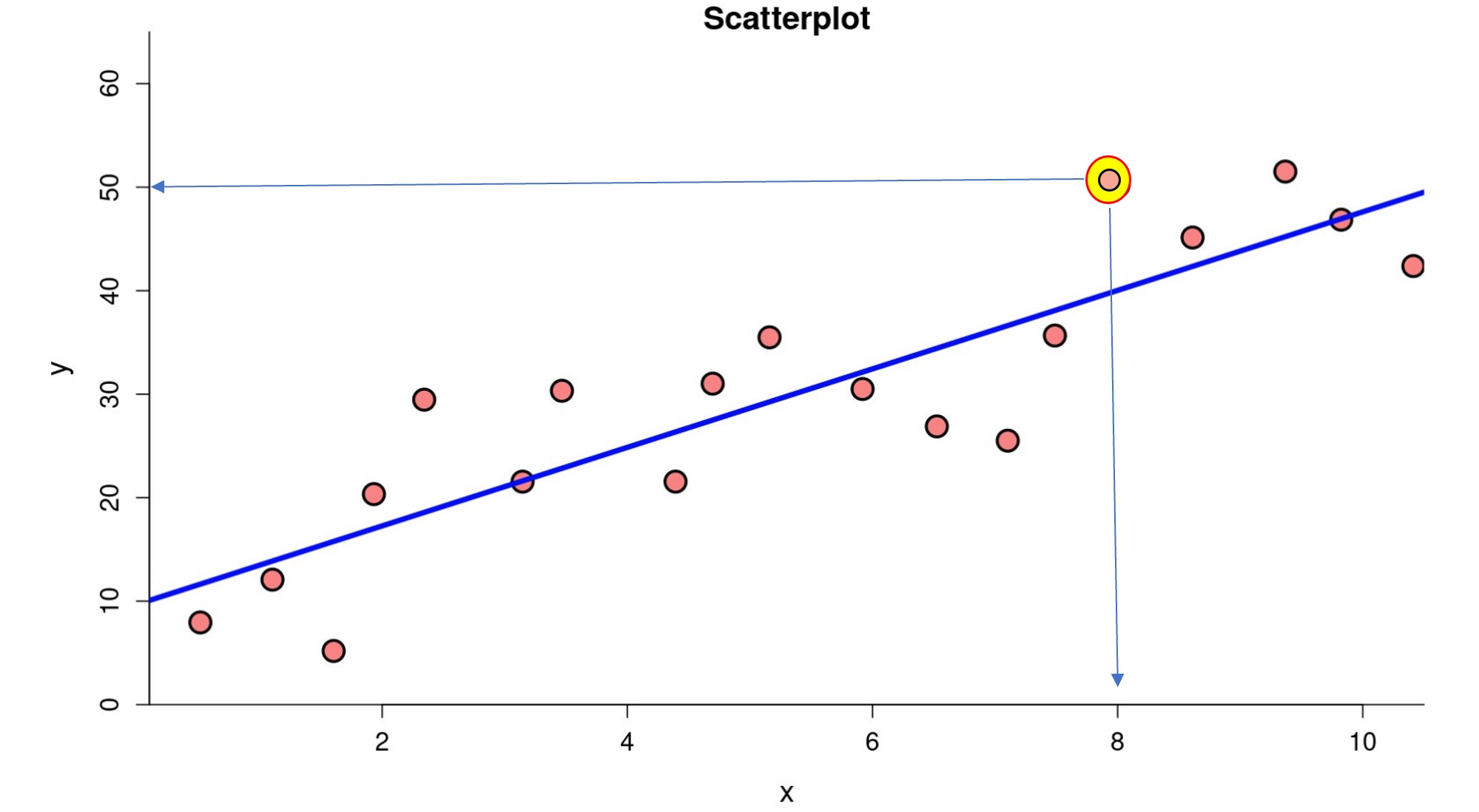
Locate the data point highlighted on the plot, located above the line of best fit. This represents an actual observation in the data set. Use this point and the line of best fit to answer the following questions.
- What is the value of the explanatory variable [latex]x[/latex]for the data point highlighted on the plot?
- What is the value of the response variable [latex]y[/latex]for the data point highlighted on the plot?
- Using the line of best fit, what appears visually to be the predicted value of the response variable [latex]\hat{y}[/latex] for this value of the explanatory variable?
- If the equation of the line of best fit is [latex]\hat{y}=10.02 + 3.48x[/latex], what is the predicted value of [latex]\hat{y}[/latex] for this value of the explanatory variable?
- Is the actual value of the response variable greater or lower than the predicted value?
- Locate a data point that lies below the line of best fit and estimate its [latex]\left(x,y\right)[/latex] coordinates.
The difference between the observed value of the response variable [latex]y[/latex] and the predicted value of the response variable [latex]\hat{y}[/latex] represents the residual for the actual data point. Some data points lie above the line of best fit and some lie below the line of best fit.
- 7. What is the residual for the highlighted data point in the scatterplot above?
- 8. Calculate the residual for the point you choose located below the line of best fit. What process did you follow?
- 9. Was the residual for a point below the line of best fit negative or positive?
- 10. Can you locate any points on the plot with a residual of zero?
Residuals and the Bad Drivers Dataset
Throughout the rest of this corequisite support activity, we’ll be focusing on the “Bad Drivers” dataset again. This dataset reports information about car crashes and contains entries corresponding to all 50 states, as well as Washington, DC. In this case, we’ll be focusing on two variables: losses (in dollars) incurred by insurance companies for collisions per insured driver and insurance premiums (in dollars).
question 4
Consider this plot of a dataset that reports information about car crashes in the United States. Each data point represents the intersection of losses by insurance companies for collisions per insured driver and insurance premiums. Both variables are in units of US dollars.
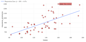
Part A: Using the plot above, what were the approximate losses incurred by insurance companies for collisions per insured driver in New Jersey?
Part B: About how much do insurance premiums cost in New Jersey?
Part C: Based on the losses in New Jersey and the line of best fit, what is the predicted average cost of insurance premiums in New Jersey?
Part D: What is the residual for New Jersey?
Part E: Fill in the blanks to interpret the residual for New Jersey.
New Jersey’s actual ____________ is _________ (greater/lower) than predicted.
question 5
In words, describe the process for finding the residual.
question 6
The following table lists information about four of the states in the dataset. Complete the table. Round to the nearest cent. Then, label the points corresponding to each of these states on the scatterplot that follows.
| State | Losses ($) | Observed Insurance Premiums ($) | Predicted Insurance Premiums ($) | Residual ($) |
| Louisiana | $194.78 | $1,281.50 | ||
| Idaho | $82.75 | $642.00 | ||
| Montana | $85.15 | $816.20 | ||
| Oklahoma | $178.86 | $881.50 |
question 7
For a given state, what is the relationship between the sign of the residual and how the observed insurance premium value compares to the predicted insurance premium value?
question 8
Of the states in the table, which state has its data point closest to the line of best fit? How can you tell from the residual?
Interpreting Residuals
There are a few different perspectives of the residual, mathematically. Let's take a look at these in Questions 9 - 12 below.
question 9
[There may be a better format for this question in OHM]
If the observed data point lies above the line of best fit, then:
a. the residual is positive/negative (circle one);
b. [latex]y < \text{ or } > \text{ or } = \hat{y}[/latex] (circle one);
c. the predicted value of the response variable is greater/less (circle one) than the observed value of the response variable; and
d. [latex]y-\hat{y} < \text{ or } > \text{ or } = 0[/latex] (circle one).
question 10
[There may be a better format for this question in OHM]
If the observed data point lies below the line of best fit, then:
- the residual is positive/negative (circle one);
- [latex]y < \text{ or } > \text{ or } = \hat{y}[/latex] (circle one);
- the predicted value of the response variable is greater/less (circle one) than the observed value of the response variable; and
- [latex]y-\hat{y} < \text{ or } > \text{ or } = 0[/latex] (circle one).
question 11
If the observed data point lies close to the line of best fit, then the residual is _______ zero.
- a) Close to
- b) Far from
question 12
If the observed data point lies far from the line of best fit, then the residual is _______ zero.
- a) Close to
- b) Far from
You've spent some good time developing an understanding of how residuals are interpreted and calculated. It's time to move to the course materials in this section to put your understanding to good use!
