goals for this section
After completing this section, you should feel comfortable performing these skills.
- Compare the variability of multiple datasets visually using histograms.
- Compare the variability of multiple datasets visually using dotplots.
- Use a data analysis tool to identify the standard deviation of a dataset.
- Calculate the variance of a dataset given standard deviation
- Use a data analysis tool to calculate variability by identifying the range of a dataset.
Click on a skill above to jump to its location in this section.
In the next activity, you will be exploring data and using the measures of center and measures of spread to describe the data. This section will introduce you to variability, which is a measure of how dispersed (spread out) the data are. You’ll learn to recognize variability in histograms and dotplots by using visual clues. You’ll also learn how to calculate measures of variability including standard deviation, variance, and range.
Comparing Variability
The variability of a dataset is often referred to as the spread of a dataset. We can visually assess variability using graphical displays such as histograms and dotplots. When answering Questions 1 – 3 below, consider whether the data appears to be more spread out from the center (greater variability) or more clustered toward the center (less variability).
Comparing Variability Using Histograms
Recall that a histogram visualizes the distribution of a quantitative variable by displaying rectangular bars representing the frequencies (height of the bar) for intervals of data values called bins (width of the bar). Variability can be judged from a histogram by examining the distance of the bars from the statistical center (mean or median) of the graph. If the variability is high, equally sized or taller bars will appear away from the center of the graph. It the variability is low, the data will appear clustered around the center.
The images below show distributions of two different datasets using histograms. The first histogram displays the distribution of responses given by parents of thirteen year old children to the question, “how much allowance do you give weekly?” The second is a distribution of the heights in inches of 31 thirteen year old boys attending the same middle-school. Use these histograms to answer Question 1 below.
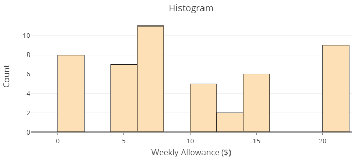
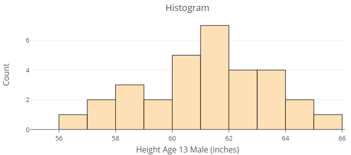
question 1
Which of the two histograms appears to have less variability? Explain.
Using Dotplots to Visually Compare Variability
A dotplot indicates the variability of the data or the extent to which each observation differs from other observations. It can be easier to visualize variability using a dotplot than using a histogram because of the individual observations visible in the dotplot. Use the side-by-side dotplots in the image below to answer Questions 2 and 3.
Ten customers rated four different smartphone apps. The customer ratings for the four different apps are shown in the following dotplots. The mean for each app is equal to 3. Even though the mean, [latex]\bar{x}[/latex], is the same for each app, the dotplots for each app look very different.
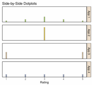
question 2
Which app has the smallest variability? In other words, in which app are the observations really close together?
a) App 1
b) App 2
c) App 3
d) App 4
question 3
Which app has the largest variability? In other words, in which app are the observations the furthest apart?
a) App 1
b) App 2
c) App 3
d) App 4
Using Technology to Obtain Descriptive Statistics
Let’s go to the technology now and recall how to load a dataset in order to describe and explore it.
For Questions 4 and 5, recall the sleep study in which you investigated whether college students’ chronotypes tend to be larks (morning people) or owls (night people) by examining graphical representations of the data. Let’s use the dataset from that study again here.
Go to the Describing and Exploring Quantitative Variables tool at https://dcmathpathways.shinyapps.io/EDA_quantitative/.
Step 1) Select the Single Group tab.
Step 2) Locate the drop-down menu under Enter Data and select From Textbook.
Step 3) Locate the drop-down menu under Dataset and select Sleep Study: Average Sleep.
question 4
The descriptive statistics are displayed in a table at the top of the webpage. Would the observations in this dataset be classified as a sample or a population?
question 5
What is the average amount of sleep (rounded to the nearest whole number) of the college students in the study?
a) 8 hours
b) 9 hours
c) 4 hours
d) 7 hours
Measures of Variability
In statistics, we are particularly interested in understanding how data are distributed and where each observation is in reference to the mean. How spread out a set of observations are is called variability (also called spread or dispersion). In the remainder of this section, we will focus on three measures of spread: standard deviation, variance, and range.
Recall
We’ll be using statistical formulas and symbols to discuss measures of variability. Take a moment to recall the formula you learned to calculate the mean of a sample. What symbols do we use to represent sample mean, summation, and sample size?
Core skill:
Standard Deviation
[perspective video — a 3-instructor video showing how to think about standard deviation as a measure of variability. Cover the parts of the formula (go into why squaring, why df if desired) but emphasize the concept of variability from std dev and variance more so than the technical use of the formula.]
Standard deviation is a measure of how spread out observations are from the mean. The symbol we use to denote standard deviation differs depending on whether we are discussing a sample or a population. We use the Greek letter [latex]\sigma[/latex] (sigma) to denote the standard deviation of a population of observations. We use the Latin letter [latex]s[/latex] to denote the standard deviation of a sample of observations.
The following formulas are used to calculate the standard deviation of a population and a sample:
Standard deviation of a population: [latex]\sigma = \sqrt{\dfrac{\sum \left(x-\mu\right)^2}{n}}[/latex]
Standard deviation of a sample: [latex]s=\sqrt{\dfrac{\sum \left(x-\bar{x}\right)^2}{n-1}}[/latex]
The following steps can be applied to calculate a standard deviation by hand.
- Calculate the mean of the population or sample.
- Take the difference between each data value and the mean. Then square each difference.
- Add up all the squared differences
- Divide by either the total number of observations in the case of a population or by 1 fewer than the total in the case of a sample.
- Take the square root of the result of the division in step 4.
Interactive example
A sample of observations is listed below. Find it’s standard deviation.
8, 7, 13, 15, 23, 18
Here is a breakdown of the formula for standard deviation of a sample, [latex]s[/latex].
[latex]s=\sqrt{\dfrac{\sum \left(x-\bar{x}\right)^2}{n-1}}[/latex]
- The distance from each observation to the mean is known as a deviation from the mean and is expressed as [latex]\left(x-\bar{x}\right)[/latex]
- The deviations from the mean are squared in the formula because some observations are above the mean, thus [latex]\left(x-\bar{x}\right)>0[/latex] (the difference is positive), and some observations are below the mean, thus [latex]\left(x-\bar{x}\right)<0[/latex] (the difference is negative). Squaring ensures the differences will each be expressed as positive distances and won’t cancel each other out when summed up.
- The [latex]\sum[/latex] symbol sums up the squared deviations for all [latex]n[/latex] observations.
- The denominator in the formula for a sample standard deviation is [latex]\left(n-1\right)[/latex] rather than [latex]n[/latex] as in the formula for the population standard deviation.
- Why do we divide by 1 fewer than the sample size, [latex]\left(n-1\right)[/latex]?
-
The answer to that is complicated but here are some ideas that may help
- The square root is taken in order to express the spread in terms of the units of the observations. Recall that we squared the differences to express them as positive distances, which resulted in squared observation units. Taking the square root can be thought of as “undoing” the earlier squaring. For example, assume that within the context in which you are working, the data are in terms of dollars. If we do not take the square root, the standard deviation will be in terms of dollars squared, which is not something commonly used.
- The standard deviation, [latex]s[/latex], represents the “typical” distance of an observation from the mean of the dataset.
Don’t worry. We will be using the DCMP Statistical Analysis Tools to calculate standard deviation for us!
Let’s practice using the tool by finding the standard deviation of the variable Average Sleep in the Sleep Study dataset.
Use a data analysis tool to identify the standard deviation of a dataset
[Worked example video – a 3-instructor video showing how to use the tool as in Questions 6 – 8 to calculate standard deviation, variance, and range with commentary on what these values imply for there being “more” or “less” variability in the data.
Go to the Describing and Exploring Quantitative Variables tool at https://dcmathpathways.shinyapps.io/EDA_quantitative/.
Step 1) Select the Single Group tab.
Step 2) Locate the drop-down menu under Enter Data and select From Textbook.
Step 3) Locate the drop-down menu under Dataset and select Sleep Study: Average Sleep.
question 6
What is the standard deviation of the average number of hours a college student in the study sleeps per week? Make sure to include units in your answer.
HintVariance
Variance is the standard deviation squared. We use the Greek letter [latex]\sigma^{2}[/latex] (sigma squared) to denote the variance of a population of observations, and we use [latex]s^{2}[/latex] to denote the variation of a sample of observations. The following formulas are used to calculate the variation of a population and a sample:
Variance of a population: [latex]\sigma^{2}=\dfrac{\sum\left(x-\mu\right)^{2}}{n}[/latex]
Variance of a sample: [latex]s^{2}=\dfrac{\sum\left(x-\bar{x}\right)^{2}}{n-1}[/latex]
Important: The Describing and Exploring Quantitative Variables tool does not calculate the variance, so you will need to use the tool to calculate the standard deviation and then square it by hand in order to get the variance.
question 7
What is the variance of the average number of hours college students in the study sleep? Round to 3 decimal places. Make sure to include units in your answer.
HintRange
The simplest way to calculate the variability of a dataset is with the range:
Range = maximum value – minimum value
or
Range = largest value – smallest value
Larger values of range indicate more variability in the data. However, the range value only utilizes two observations in the entire dataset to measure variability. This is not an ideal measure of spread, but when used in combination with other measures of spread, it can help us gain a clearer understanding of the spread of a distribution.
question 8
What is the range of the average number of hours a college student in the study sleeps per week?
HintSummary
In this section, you’ve learned about variability in a dataset in preparation for exploring data via the measures of center and spread. Let’s summarize where these skills showed up in the material.
- In Questions 1, 2, and 3, you visually assessed the differences in variability, given comparative histograms or dotplots.
- In Questions 4 and 5, you gained experience using the summary statistics feature of the Describing and Exploring Quantitative Variables tool.
- In questions 6 – 8, you used technology to calculate measures of variability: standard deviation, variance, and range.
Exploring the measures of center and spread to describe data is a necessary skill for completing the next activity. If you feel comfortable with these skills, it’s time to move on!
-
- Why do we divide by 1 fewer than the sample size, [latex]\left(n-1\right)[/latex]?
