Learning Goals
At the end of this page, you should feel comfortable performing these skills:
- Identify the explanatory and response variables in a given scenario.
- Identify when a linear regression analysis might be appropriate.
- Use technology to perform a least squares regression analysis.
Bivariate Data
In the upcoming activity, you will need to identify the explanatory and response variable given a scenario and understand when linear regression analysis might be appropriate. In this page, you’ll prepare for that by looking carefully at definitions, applying the definitions in given scenarios, and seeing specific situations in which data may or may not be related linearly.
Often, we do statistical studies to find relationships between two or more variables that can help us to better predict future outcomes and perhaps make changes that will improve our lives.
In the next activity, we will be focusing on studies and relationships involving two quantitative variables. In each dataset, the two variables will be linked because both observations will be measured from the same individual or unit.
These types of linked data are called bivariate data and are often presented in scatterplots. Bivariate data are defined as pairs of data values, where each pair consists of two different measurements that come from the same individual or unit.
See the video below for a quick explanation.
Video Placement
[Perspective Video: ] A short video (1 minute or less) that shows graphs with common examples of bivariate data — just showing the placement of explanatory and response variables on the axis and showing how each data point on a scatterplot indicates one input/response observation in the data set. Examples might include miles driven over gas prices, revenue over marketing expenditures, annual income over total years of school, etc.
Now that you have the idea of two related quantitative variables, read on to see how to determine the nature of the two variables in an existing bivariate data set or study of bivariate data. The key idea is that one of the variables will measure the outcome of the study. It will be dependent upon the other variable.
Explanatory and Response Variables
A teacher wonders if “number of absences per semester” is related to “academic performance” for students in her classes. She might look back on her class records from previous semesters and generate a dataset by observing both the final overall average grade and total number of missed classes for each student in a random sample of students. This is an example of a bivariate dataset.
When working with a bivariate dataset, there are two variables to consider:
- The explanatory variable ([latex]x[/latex]) is the variable that is thought to explain or predict the response variable of a study.
- The response variable ([latex]y[/latex]) measures the outcome of interest in the study. This variable is thought to depend in some way on the explanatory variable. It is often referred to as the “variable of interest” for the researcher. (In your previous math classes this variable may have been referred to as the dependent variable.)
In this example, the outcome the teacher is most interested in is how well her students will do in her class, so the response variable is Overall Average Grade. The other variable, Number of Absences, is the explanatory variable.
Identifying explanatory and response variables can sometimes be difficult. When trying to identify explanatory and response variables, make sure to carefully read the scenario and keep the following phrases in mind:
Explanatory is used to predict Response
(or calculate)
(or determine)
It is good practice to identify both variables and then ask, “Which one is the main outcome or focus of the study?” This variable will be the response variable, and the other variable will be the explanatory variable. When reading a pre-existing study, carefully read the context of the study to identify which variable is being used to explain (the explanatory variable) an outcome or response (the response variable).
example
[This is a good place to use socially equitable or topical data to replace this common example]
Scenario 1. Suppose a chamber of commerce wants to investigate sales in an historic shopping district under various weather conditions. They choose to keep track of the total in-person sales by day and daily high temperatures.
Which of these two variables Daily Sales or Daily High Temp is the response variable? Which is the explanatory variable?
Scenario 2. Later, the chamber of commerce wishes to explore whether the daily number of shoppers in the district is related to the daytime precipitation. They collect the number of inches of precipitation that fell between 9am and 6pm each day for a certain time period and also the number of times a person crossed through the gate to the main shopping courtyard.
Which of these two variables, Daily Precipitation or Number of Shoppers is the response variable? Which is the explanatory variable?
We’ll see shortly that both variables present in a bivariate data set will need to be quantitative in order to determine a linear relationship. Note for example that both of the scenarios in the example above included only quantitative variables. To define explanatory and response variables in any bivariate data set, when the study seeks only a correlation, both variables need not be quantitative. Keep this in mind as you answer Questions 1 and 2 below to define and identify explanatory and response variables in a given scenario.
question 1
True or False: The response variable can be thought of as the predicted variable or outcome.
- a) True
- b) False
question 2
A researcher wonders if a new cancer treatment leads to a higher five-year survival rate for people diagnosed with a certain type of lung cancer. She creates an experiment where the experimental group gets the new treatment and the control group gets the traditional treatment. After five years, she gathers data on the people in each group to see which cancer patients survived and which did not.
Part A: Identify the explanatory variable. Select the best answer.
- a) Survival status of the patient after five years (survived or did not survive)
- b) Treatment status of the patient (control group or experimental group)
- c) Cancer status (diagnosed with cancer or no cancer)
- d) The years of study (1, 2, 3, 4, or 5)
Part B: Identify the response variable. Select the best answer.
- a) Survival status of the patient after five years (survived or did not survive)
- b) Treatment status of the patient (control group or new treatment group)
- c) Cancer status (diagnosed with cancer or no cancer)
- d) The years of study (1, 2, 3, 4, or 5)
Linear Relationships
A method we will use to make predictions about missing observations or future observations in bivariate data is called Least Squares Regression (LSR) analysis. The language might seem intimidating at first, but the ideas are quite straightforward, especially with examples to illustrate each new term. For example, LSR analysis can also be described as linear modeling, where we determine the equation of a line of best fit to make predictions based on an existing dataset. In this type of analysis, both the explanatory and response variables must be quantitative, since the linear model requires numerical values in its calculations.
Video Placement
[A 3-Instructor Perspective Video: A description and explanation of least squares regression using a scatterplot, line of best fit, vertical error (residuals), and linear equation. Note in the video that both variables must be quantitative in order to perform a linear analysis. It should end with an explanation of common statistical notation for slope and y-intercept, showing that the equation for the line of best fit is the same equation students learned in algebra I as y=mx+b, except that since this line is a rough representation of the data set, the outcome is merely a prediction, thus denoted [latex]\hat{y}[/latex].
Line of Best Fit
The line of best fit is simply the best line that describes the data points. For real data with natural deviations, the line cannot go through all of the points. In fact, very often, the line does not go through any of the data points.
Since no line will be perfect, the best we can do is minimize its error. In this class, we will do this by minimizing the sum total of the squared vertical errors from all data points to the line. This is why the line of best fit is also called the Least Squares Regression Line (LSRL).
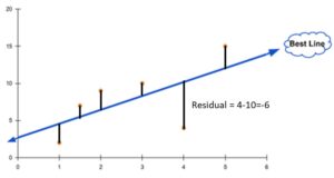
The vertical error associated with each data point is called the residual of that observation. This error, illustrated by the length of the vertical line, represents how far off a prediction calculated from the line is compared to the actual, observed [latex]y[/latex] value; the larger the line, the greater the error associated with that particular observation.
Note: For data points that are above the line of best fit, the residuals are positive, and for data points that are below the line, the residuals are negative.
The equation for the line of best fit is very similar to one you may have seen in a previous math class:
[latex]\hat{y} = a+bx[/latex]
where [latex]\hat{y}[/latex] is the general predicted value of the response variable (pronounced y-hat), a is the estimated value of the y-intercept, and [latex]b[/latex] is the estimated slope.
While the actual process of finding the line of best fit might seem complicated, the concept of line of best fit is very straightforward. We can use technology to take care of long and tedious calculations.
When is LSR Analysis Appropriate?
As you answer Questions 3 and 4, keep in mind that in order to create a linear model during LSR analysis, both of the variables in the bivariate data must be quantitative.
Question 3
Which of the following questions could be explored using LSR analysis involving bivariate data? Select all that apply.
- a) Could the number of cigarettes a person smokes per day be used to predict a person’s lifespan?
- b) Does our race, ethnicity, and/or gender impact the likelihood that we will be treated fairly when seeking a loan, medical treatment, or pursuing an educational degree?
- c) Does the amount of sleep we get per day have an impact on our weight?
- d) Is there are association between the type of pet people own and their level of general happiness?
Question 4
Can we use LSR analysis to better understand the data generated from the experiment in Question 2? Select the best answer.
- a) Yes, if it is a well-designed experiment.
- b) Yes, because LSR analysis can be used to understand and make better predictions for all datasets.
- c) No, because at least one of the variables is categorical.
Performing LSR Analysis
Now let’s put everything you’ve seen in this activity together to perform an LSR analysis using technology. See the example below for guidance, then answer Question 5.
Video Placement
[Worked Example: A 3-instructor worked example that follows the structure of Question 5. This would be an excellent placement for a social justice or inclusion topic. The data should be appropriate for LSR, it should identify the explanatory and response variables, and it should be used to create and visually inspect a scatterplot using technology. It should then use technology to calculate a line of best fit and the correlation coefficient. ]
Now it’s your turn to try.
Question 5
A scientist gathered data on the striped ground cricket to see if ground temperature (measured in degrees Fahrenheit) can be predicted by the number of chirps the cricket makes per second (measured in number of wing vibrations per second). After collecting the data, he could create a scatterplot to understand if there is a positive linear trend.
Part A: Can LSR analysis be used to examine these data? Select the best answer.
- a) No, because this is an observational study and not an experiment.
- b) Yes, because these are bivariate data and both variables are quantitative (and it does not matter that this was an observational study).
Part B: Identify the explanatory variable. Select the best answer.
- a) Ground temperature
- b) Number of crickets
- c) Time of day
- d) Number of chirps per second
Part C: Identify the response variable. Select the best answer.
- a) Ground temperature
- b) Number of crickets
- c) Time of day
- d) Number of chirps per second
The following is a chart of the data the scientist collected to help him answer his question.
| Chirps per second | Temperature in degrees Fahrenheit |
| 20 | 88.6 |
| 16 | 71.6 |
| 19.8 | 93.3 |
| 18.4 | 84.3 |
| 17.1 | 80.6 |
| 15.5 | 75.2 |
| 14.7 | 69.7 |
| 17.1 | 82 |
| 15.4 | 69.4 |
| 16.2 | 83.3 |
| 15 | 79.6 |
| 17.2 | 82.6 |
| 16 | 80.6 |
| 17 | 83.5 |
| 14.4 | 76.3 |
Go to the Linear Regression tool at https://dcmathpathways.shinyapps.io/LinearRegression/ and plot the data using the following steps: under “Enter Data,” select “Enter Own;” name the x (explanatory) and y (response) variables appropriately; copy and paste the data from the table (make sure the explanatory variable is in the first column and the response variable is in the second column); under “Plot Options,” select “Regression Line;” and select “Submit Data.”
Part D: Does the scatterplot look fairly linear?
Part E: What is the equation of the line of best fit?
Part F: What is the value of the correlation coefficient?
You’ve seen some of these ideas before in Forming Connections [5A]. Review those notes now to answer Question 6. Make sure to have your answer for Question 6 handy as you begin the upcoming Forming Connections activity!
Question 6
Look over your notes from In-Class Activity 5.A. Write down three different examples where you noted an explanatory variable that can be used to predict a response variable and where both variables are quantitative. One scenario should have a positive association, one should have a negative association, and one should have no association or almost no association.
You will be looking at your three examples at the beginning of the upcoming Forming Connections. Make sure you have your examples available at the start of that activity.
Summary
In this What to Know page, you learned to recognize when a linear regression analysis is appropriate, how to identify the explanatory and response variables in bivariate data, and how to calculate the line of best fit. Let’s summarize the skills as you saw them in each question.
- In Questions 3, 4, and Question 5 Part A, you identified when a linear regression analysis might be appropriate.
- In Questions 1, 2, and Question 5 Parts B and C, you identified the explanatory and response variables in a given scenario.
- In Question 5 Parts D through F, you calculated the line of best fit and wrote it using proper notation.
If you feel comfortable with these ideas, it’s time to move on to Forming Connections in the next activity!
