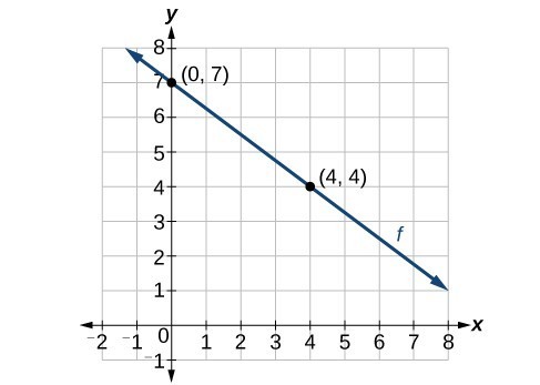
Now that we have written equations for linear functions in both the slope-intercept form and the point-slope form, we can choose which method to use based on the information we are given. That information may be provided in the form of a graph, a point and a slope, two points, and so on. Look at the graph of the function f in Figure 8.

Figure 8
We are not given the slope of the line, but we can choose any two points on the line to find the slope. Let’s choose (0, 7) and (4, 4). We can use these points to calculate the slope.
Now we can substitute the slope and the coordinates of one of the points into the point-slope form.
If we want to rewrite the equation in the slope-intercept form, we would find

Figure 9
If we wanted to find the slope-intercept form without first writing the point-slope form, we could have recognized that the line crosses the y-axis when the output value is 7. Therefore, b = 7. We now have the initial value b and the slope m so we can substitute m and b into the slope-intercept form of a line.
So the function is [latex]f\left(x\right)=-\frac{3}{4}x+7[/latex], and the linear equation would be [latex]y=-\frac{3}{4}x+7[/latex].
How To: Given the graph of a linear function, write an equation to represent the function.
- Identify two points on the line.
- Use the two points to calculate the slope.
- Determine where the line crosses the y-axis to identify the y-intercept by visual inspection.
- Substitute the slope and y-intercept into the slope-intercept form of a line equation.
Example 7: Writing an Equation for a Linear Function
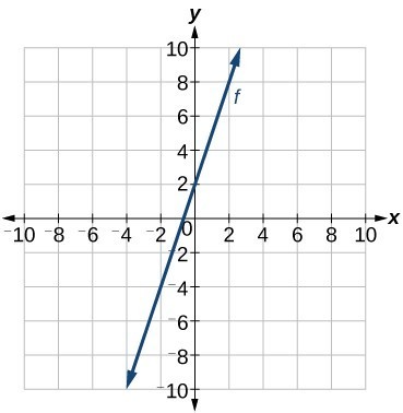
Write an equation for a linear function given a graph of f shown in Figure 10.

Figure 10
Solution
Identify two points on the line, such as (0, 2) and (–2, –4). Use the points to calculate the slope.
Substitute the slope and the coordinates of one of the points into the point-slope form.
We can use algebra to rewrite the equation in the slope-intercept form.
Example 8: Writing an Equation for a Linear Cost Function
Suppose Ben starts a company in which he incurs a fixed cost of $1,250 per month for the overhead, which includes his office rent. His production costs are $37.50 per item. Write a linear function C where C(x) is the cost for x items produced in a given month.
Solution
The fixed cost is present every month, $1,250. The costs that can vary include the cost to produce each item, which is $37.50 for Ben. The variable cost, called the marginal cost, is represented by 37.5. The cost Ben incurs is the sum of these two costs, represented by [latex]C\left(x\right)=1250+37.5x[/latex].
Analysis of the Solution
If Ben produces 100 items in a month, his monthly cost is represented by
So his monthly cost would be $5,000.
Example 9: Writing an Equation for a Linear Function Given Two Points
If f is a linear function, with [latex]f\left(3\right)=-2[/latex] , and [latex]f\left(8\right)=1[/latex], find an equation for the function in slope-intercept form.
Solution
We can write the given points using coordinates.
We can then use the points to calculate the slope.
Substitute the slope and the coordinates of one of the points into the point-slope form.
We can use algebra to rewrite the equation in the slope-intercept form.
Try It 5
If [latex]f\left(x\right)[/latex] is a linear function, with [latex]f\left(2\right)=-11[/latex], and [latex]f\left(4\right)=-25[/latex], find an equation for the function in slope-intercept form.
Modeling Real-World Problems with Linear Functions
In the real world, problems are not always explicitly stated in terms of a function or represented with a graph. Fortunately, we can analyze the problem by first representing it as a linear function and then interpreting the components of the function. As long as we know, or can figure out, the initial value and the rate of change of a linear function, we can solve many different kinds of real-world problems.
How To: Given a linear function f and the initial value and rate of change, evaluate f(c).
- Determine the initial value and the rate of change (slope).
- Substitute the values into [latex]f\left(x\right)=mx+b[/latex].
- Evaluate the function at [latex]x=c[/latex].
Example 10: Using a Linear Function to Determine the Number of Songs in a Music Collection
Marcus currently has 200 songs in his music collection. Every month, he adds 15 new songs. Write a formula for the number of songs, N, in his collection as a function of time, t, the number of months. How many songs will he own in a year?
Solution
The initial value for this function is 200 because he currently owns 200 songs, so N(0) = 200, which means that b = 200.

Figure 12
The number of songs increases by 15 songs per month, so the rate of change is 15 songs per month. Therefore we know that m = 15. We can substitute the initial value and the rate of change into the slope-intercept form of a line.
We can write the formula [latex]N\left(t\right)=15t+200[/latex].
With this formula, we can then predict how many songs Marcus will have in 1 year (12 months). In other words, we can evaluate the function at t = 12.
Marcus will have 380 songs in 12 months.
Analysis of the Solution
Notice that N is an increasing linear function. As the input (the number of months) increases, the output (number of songs) increases as well.
Example 11: Using a Linear Function to Calculate Salary Plus Commission
Working as an insurance salesperson, Ilya earns a base salary plus a commission on each new policy. Therefore, Ilya’s weekly income, I, depends on the number of new policies, n, he sells during the week. Last week he sold 3 new policies, and earned $760 for the week. The week before, he sold 5 new policies and earned $920. Find an equation for I(n), and interpret the meaning of the components of the equation.
Solution
The given information gives us two input-output pairs: (3, 760) and (5, 920). We start by finding the rate of change.
Keeping track of units can help us interpret this quantity. Income increased by $160 when the number of policies increased by 2, so the rate of change is $80 per policy. Therefore, Ilya earns a commission of $80 for each policy sold during the week.
We can then solve for the initial value.
The value of b is the starting value for the function and represents Ilya’s income when n = 0, or when no new policies are sold. We can interpret this as Ilya’s base salary for the week, which does not depend upon the number of policies sold.
We can now write the final equation.
Our final interpretation is that Ilya’s base salary is $520 per week and he earns an additional $80 commission for each policy sold.
Example 12: Using Tabular Form to Write an Equation for a Linear Function
The table below relates the number of rats in a population to time, in weeks. Use the table to write a linear equation.
| w, number of weeks | 0 | 2 | 4 | 6 |
| P(w), number of rats | 1000 | 1080 | 1160 | 1240 |
Solution
We can see from the table that the initial value for the number of rats is 1000, so b = 1000.
Rather than solving for m, we can tell from looking at the table that the population increases by 80 for every 2 weeks that pass. This means that the rate of change is 80 rats per 2 weeks, which can be simplified to 40 rats per week.
If we did not notice the rate of change from the table we could still solve for the slope using any two points from the table. For example, using (2, 1080) and (6, 1240)
Q & A
Is the initial value always provided in a table of values like the table in Example 12?
No. Sometimes the initial value is provided in a table of values, but sometimes it is not. If you see an input of 0, then the initial value would be the corresponding output. If the initial value is not provided because there is no value of input on the table equal to 0, find the slope, substitute one coordinate pair and the slope into [latex]f\left(x\right)=mx+b[/latex], and solve for b.
Try It 6
A new plant food was introduced to a young tree to test its effect on the height of the tree. The table below shows the height of the tree, in feet, x months since the measurements began. Write a linear function, H(x), where x is the number of months since the start of the experiment.
| x | 0 | 2 | 4 | 8 | 12 |
| H(x) | 12.5 | 13.5 | 14.5 | 16.5 | 18.5 |
Candela Citations
- Precalculus. Authored by: Jay Abramson, et al.. Provided by: OpenStax. Located at: http://cnx.org/contents/fd53eae1-fa23-47c7-bb1b-972349835c3c@5.175. License: CC BY: Attribution. License Terms: Download For Free at : http://cnx.org/contents/fd53eae1-fa23-47c7-bb1b-972349835c3c@5.175.
Analysis of the Solution
This makes sense because we can see from Figure 11 that the line crosses the y-axis at the point (0, 2), which is the y-intercept, so b = 2.
Figure 11