Learning Outcomes
- Find the average rate of change of a function.
- Use a graph to determine where a function is increasing, decreasing, or constant.
- Use a graph to locate local and absolute maxima and local minima.
- Combine functions using algebraic operations.
- Create a new function by composition of functions.
- Evaluate composite functions.
- Find the domain of a composite function.
- Decompose a composite function into its component functions.
Rates of Change
Gasoline costs have experienced some wild fluctuations over the last several decades. The table below[1] lists the average cost, in dollars, of a gallon of gasoline for the years 2005–2012. The cost of gasoline can be considered as a function of year.
| [latex]y[/latex] | 2005 | 2006 | 2007 | 2008 | 2009 | 2010 | 2011 | 2012 |
| [latex]C\left(y\right)[/latex] | 2.31 | 2.62 | 2.84 | 3.30 | 2.41 | 2.84 | 3.58 | 3.68 |
If we were interested only in how the gasoline prices changed between 2005 and 2012, we could compute that the cost per gallon had increased from $2.31 to $3.68, an increase of $1.37. While this is interesting, it might be more useful to look at how much the price changed per year. In this section, we will investigate changes such as these.
Finding the Average Rate of Change of a Function
The price change per year is a rate of change because it describes how an output quantity changes relative to the change in the input quantity. We can see that the price of gasoline in the table above did not change by the same amount each year, so the rate of change was not constant. If we use only the beginning and ending data, we would be finding the average rate of change over the specified period of time. To find the average rate of change, we divide the change in the output value by the change in the input value.
The Greek letter [latex]\Delta[/latex] (delta) signifies the change in a quantity; we read the ratio as “delta-y over delta-x” or “the change in [latex]y[/latex] divided by the change in [latex]x[/latex].” Occasionally we write [latex]\Delta f[/latex] instead of [latex]\Delta y[/latex], which still represents the change in the function’s output value resulting from a change to its input value. It does not mean we are changing the function into some other function.
In our example, the gasoline price increased by $1.37 from 2005 to 2012. Over 7 years, the average rate of change was
On average, the price of gas increased by about 19.6¢ each year.
Other examples of rates of change include:
- A population of rats increasing by 40 rats per week
- A car traveling 68 miles per hour (distance traveled changes by 68 miles each hour as time passes)
- A car driving 27 miles per gallon (distance traveled changes by 27 miles for each gallon)
- The current through an electrical circuit increasing by 0.125 amperes for every volt of increased voltage
- The amount of money in a college account decreasing by $4,000 per quarter
A General Note: Rate of Change
A rate of change describes how an output quantity changes relative to the change in the input quantity. The units on a rate of change are “output units per input units.”
The average rate of change between two input values is the total change of the function values (output values) divided by the change in the input values.
How To: Given the value of a function at different points, calculate the average rate of change of a function for the interval between two values [latex]{x}_{1}[/latex] and [latex]{x}_{2}[/latex].
- Calculate the difference [latex]{y}_{2}-{y}_{1}=\Delta y[/latex].
- Calculate the difference [latex]{x}_{2}-{x}_{1}=\Delta x[/latex].
- Find the ratio [latex]\frac{\Delta y}{\Delta x}[/latex].
Example 1: Computing an Average Rate of Change
Using the data in the table below, find the average rate of change of the price of gasoline between 2007 and 2009.
| [latex]y[/latex] | 2005 | 2006 | 2007 | 2008 | 2009 | 2010 | 2011 | 2012 |
| [latex]C\left(y\right)[/latex] | 2.31 | 2.62 | 2.84 | 3.30 | 2.41 | 2.84 | 3.58 | 3.68 |
The following video provides another example of how to find the average rate of change between two points from a table of values.
Try It
Using the data in the table below, find the average rate of change between 2005 and 2010.
| [latex]y[/latex] | 2005 | 2006 | 2007 | 2008 | 2009 | 2010 | 2011 | 2012 |
| [latex]C\left(y\right)[/latex] | 2.31 | 2.62 | 2.84 | 3.30 | 2.41 | 2.84 | 3.58 | 3.68 |
Example 2: Computing Average Rate of Change from a Graph
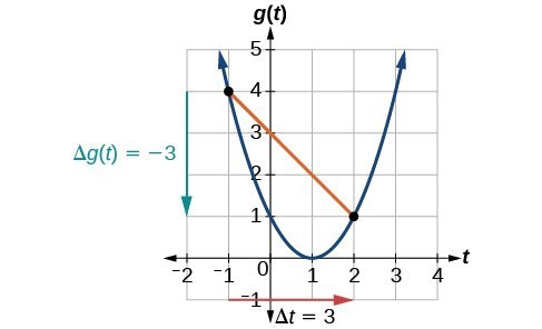
Given the function [latex]g\left(t\right)[/latex] shown in Figure 1, find the average rate of change on the interval [latex]\left[-1,2\right][/latex].
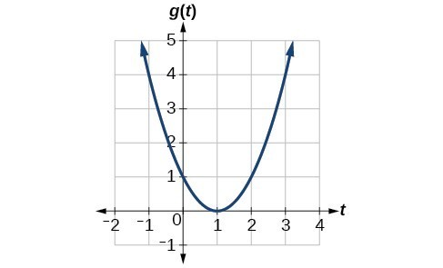
Figure 1
Example 3: Computing Average Rate of Change from a Table
After picking up a friend who lives 10 miles away, Anna records her distance from home over time. The values are shown in the table below. Find her average speed over the first 6 hours.
| t (hours) | 0 | 1 | 2 | 3 | 4 | 5 | 6 | 7 |
| D(t) (miles) | 10 | 55 | 90 | 153 | 214 | 240 | 292 | 300 |
Example 4: Computing Average Rate of Change for a Function Expressed as a Formula
Compute the average rate of change of [latex]f\left(x\right)={x}^{2}-\frac{1}{x}[/latex] on the interval [latex]\text{[2,}\text{4].}[/latex]
The following video provides another example of finding the average rate of change of a function given a formula and an interval.
Try It
Find the average rate of change of [latex]f\left(x\right)=x - 2\sqrt{x}[/latex] on the interval [latex]\left[1,9\right][/latex].
Try It
Example 5: Finding the Average Rate of Change of a Force
The electrostatic force [latex]F[/latex], measured in newtons, between two charged particles can be related to the distance between the particles [latex]d[/latex], in centimeters, by the formula [latex]F\left(d\right)=\frac{2}{{d}^{2}}[/latex]. Find the average rate of change of force if the distance between the particles is increased from 2 cm to 6 cm.
Example 6: Finding an Average Rate of Change as an Expression
Find the average rate of change of [latex]g\left(t\right)={t}^{2}+3t+1[/latex] on the interval [latex]\left[0,a\right][/latex]. The answer will be an expression involving [latex]a[/latex].
Try It
Find the average rate of change of [latex]f\left(x\right)={x}^{2}+2x - 8[/latex] on the interval [latex]\left[5,a\right][/latex].
As part of exploring how functions change, we can identify intervals over which the function is changing in specific ways. We say that a function is increasing on an interval if the function values increase as the input values increase within that interval. Similarly, a function is decreasing on an interval if the function values decrease as the input values increase over that interval. The average rate of change of an increasing function is positive, and the average rate of change of a decreasing function is negative. Figure 3 shows examples of increasing and decreasing intervals on a function.
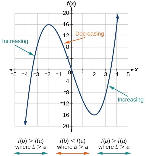
Figure 3. The function [latex]f\left(x\right)={x}^{3}-12x[/latex] is increasing on [latex]\left(-\infty \text{,}-\text{2}\right){{\cup }^{\text{ }}}^{\text{ }}\left(2,\infty \right)[/latex] and is decreasing on [latex]\left(-2\text{,}2\right)[/latex].
This video further explains how to find where a function is increasing or decreasing.
While some functions are increasing (or decreasing) over their entire domain, many others are not. A value of the input where a function changes from increasing to decreasing (as we go from left to right, that is, as the input variable increases) is called a local maximum. If a function has more than one, we say it has local maxima. Similarly, a value of the input where a function changes from decreasing to increasing as the input variable increases is called a local minimum. The plural form is “local minima.” Together, local maxima and minima are called local extrema, or local extreme values, of the function. (The singular form is “extremum.”) Often, the term local is replaced by the term relative. In this text, we will use the term local.
Clearly, a function is neither increasing nor decreasing on an interval where it is constant. A function is also neither increasing nor decreasing at extrema. Note that we have to speak of local extrema, because any given local extremum as defined here is not necessarily the highest maximum or lowest minimum in the function’s entire domain.
For the function in Figure 4, the local maximum is 16, and it occurs at [latex]x=-2[/latex]. The local minimum is [latex]-16[/latex] and it occurs at [latex]x=2[/latex].
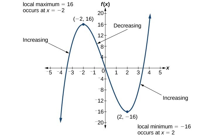
Figure 4
To locate the local maxima and minima from a graph, we need to observe the graph to determine where the graph attains its highest and lowest points, respectively, within an open interval. Like the summit of a roller coaster, the graph of a function is higher at a local maximum than at nearby points on both sides. The graph will also be lower at a local minimum than at neighboring points. Figure 5 illustrates these ideas for a local maximum.
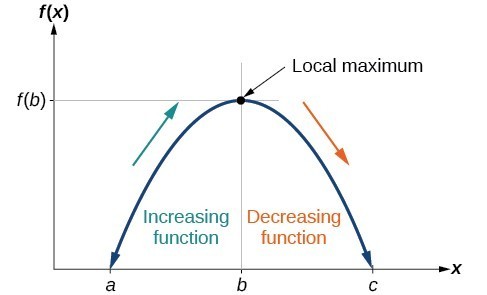
Figure 5. Definition of a local maximum.
These observations lead us to a formal definition of local extrema.
A General Note: Local Minima and Local Maxima
A function [latex]f[/latex] is an increasing function on an open interval if [latex]f\left(b\right)>f\left(a\right)[/latex] for any two input values [latex]a[/latex] and [latex]b[/latex] in the given interval where [latex]b>a[/latex].
A function [latex]f[/latex] is a decreasing function on an open interval if [latex]f\left(b\right)
A function [latex]f[/latex] has a local maximum at [latex]x=b[/latex] if there exists an interval [latex]\left(a,c\right)[/latex] with [latex]a
Example 7: Finding Increasing and Decreasing Intervals on a Graph
Given the function [latex]p\left(t\right)[/latex] in the graph below, identify the intervals on which the function appears to be increasing.
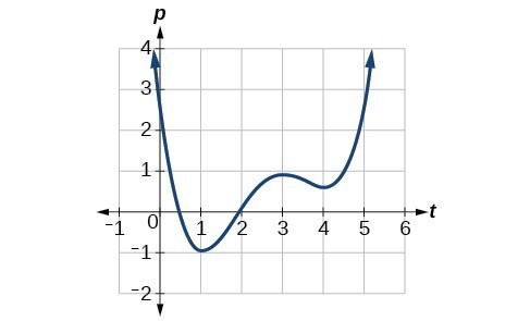
Figure 6
Example 8: Finding Local Extrema from a Graph
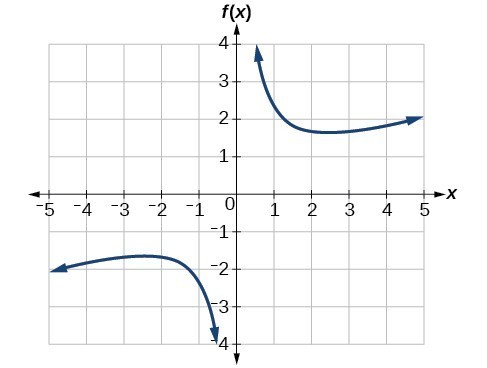
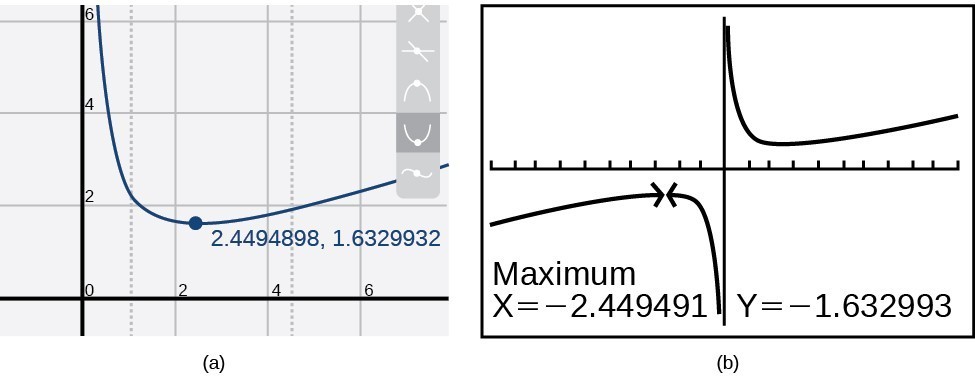
Graph the function [latex]f\left(x\right)=\frac{2}{x}+\frac{x}{3}[/latex]. Then use the graph to estimate the local extrema of the function and to determine the intervals on which the function is increasing.
Try It
Graph the function [latex]f\left(x\right)={x}^{3}-6{x}^{2}-15x+20[/latex] to estimate the local extrema of the function. Use these to determine the intervals on which the function is increasing and decreasing.

Try It
Example 9: Finding Local Maxima and Minima from a Graph
For the function [latex]f[/latex] whose graph is shown in Figure 9, find all local maxima and minima.
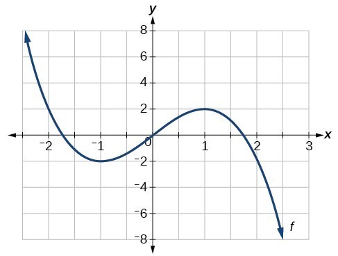
Figure 9
Analyzing the Toolkit Functions for Increasing or Decreasing Intervals
We will now return to our toolkit functions and discuss their graphical behavior in the table below.
| Function | Increasing/Decreasing | Example |
|---|---|---|
| Constant Function
[latex]f\left(x\right)={c}[/latex] |
Neither increasing nor decreasing | 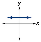 |
| Identity Function
[latex]f\left(x\right)={x}[/latex] |
Increasing | 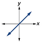 |
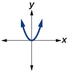
| Quadratic Function
[latex]f\left(x\right)={x}^{2}[/latex] |
Increasing on [latex]\left(0,\infty\right)[/latex]
Decreasing on [latex]\left(-\infty,0\right)[/latex] Minimum at [latex]x=0[/latex] |
 |
| Cubic Function
[latex]f\left(x\right)={x}^{3}[/latex] |
Increasing | 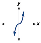 |
| Reciprocal
[latex]f\left(x\right)=\frac{1}{x}[/latex] |
Decreasing [latex]\left(-\infty,0\right)\cup\left(0,\infty\right)[/latex] | 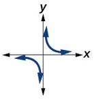 |
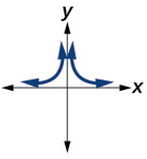
| Reciprocal Squared
[latex]f\left(x\right)=\frac{1}{{x}^{2}}[/latex] |
Increasing on [latex]\left(-\infty,0\right)[/latex]
Decreasing on [latex]\left(0,\infty\right)[/latex] |
 |
| Cube Root
[latex]f\left(x\right)=\sqrt[3]{x}[/latex]
|
Increasing | 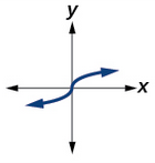 |
| Square Root
[latex]f\left(x\right)=\sqrt{x}[/latex] |
Increasing on [latex]\left(0,\infty\right)[/latex] | 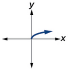 |
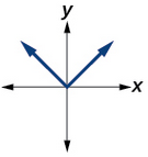
| Absolute Value
[latex]f\left(x\right)=|x|[/latex] |
Increasing on [latex]\left(0,\infty\right)[/latex]
Decreasing on [latex]\left(-\infty,0\right)[/latex] |
 |
Composition of Functions
Suppose we want to calculate how much it costs to heat a house on a particular day of the year. The cost to heat a house will depend on the average daily temperature, and in turn, the average daily temperature depends on the particular day of the year. Notice how we have just defined two relationships: The cost depends on the temperature, and the temperature depends on the day.

Figure 1
Using descriptive variables, we can notate these two functions. The function [latex]C\left(T\right)[/latex] gives the cost [latex]C[/latex] of heating a house for a given average daily temperature in [latex]T[/latex] degrees Celsius. The function [latex]T\left(d\right)[/latex] gives the average daily temperature on day [latex]d[/latex] of the year. For any given day, [latex]\text{Cost}=C\left(T\left(d\right)\right)[/latex] means that the cost depends on the temperature, which in turns depends on the day of the year. Thus, we can evaluate the cost function at the temperature [latex]T\left(d\right)[/latex]. For example, we could evaluate [latex]T\left(5\right)[/latex] to determine the average daily temperature on the 5th day of the year. Then, we could evaluate the cost function at that temperature. We would write [latex]C\left(T\left(5\right)\right)[/latex].
By combining these two relationships into one function, we have performed function composition, which is the focus of this section.
Combining Functions Using Algebraic Operations
Function composition is only one way to combine existing functions. Another way is to carry out the usual algebraic operations on functions, such as addition, subtraction, multiplication and division. We do this by performing the operations with the function outputs, defining the result as the output of our new function.
Suppose we need to add two columns of numbers that represent a husband and wife’s separate annual incomes over a period of years, with the result being their total household income. We want to do this for every year, adding only that year’s incomes and then collecting all the data in a new column. If [latex]w\left(y\right)[/latex] is the wife’s income and [latex]h\left(y\right)[/latex] is the husband’s income in year [latex]y[/latex], and we want [latex]T[/latex] to represent the total income, then we can define a new function.
If this holds true for every year, then we can focus on the relation between the functions without reference to a year and write
Just as for this sum of two functions, we can define difference, product, and ratio functions for any pair of functions that have the same kinds of inputs (not necessarily numbers) and also the same kinds of outputs (which do have to be numbers so that the usual operations of algebra can apply to them, and which also must have the same units or no units when we add and subtract). In this way, we can think of adding, subtracting, multiplying, and dividing functions.
For two functions [latex]f\left(x\right)[/latex] and [latex]g\left(x\right)[/latex] with real number outputs, we define new functions [latex]f+g,f-g,fg[/latex], and [latex]\frac{f}{g}[/latex] by the relations
Example 1: Performing Algebraic Operations on Functions
Find and simplify the functions [latex]\left(g-f\right)\left(x\right)[/latex] and [latex]\left(\frac{g}{f}\right)\left(x\right)[/latex], given [latex]f\left(x\right)=x - 1[/latex] and [latex]g\left(x\right)={x}^{2}-1[/latex]. Are they the same function?
Try It
Find and simplify the functions [latex]\left(fg\right)\left(x\right)[/latex] and [latex]\left(f-g\right)\left(x\right)[/latex].
Are they the same function?
Create a Function by Composition of Functions
Performing algebraic operations on functions combines them into a new function, but we can also create functions by composing functions. When we wanted to compute a heating cost from a day of the year, we created a new function that takes a day as input and yields a cost as output. The process of combining functions so that the output of one function becomes the input of another is known as a composition of functions. The resulting function is known as a composite function. We represent this combination by the following notation:
[latex]\left(f\circ g\right)\left(x\right)=f\left(g\left(x\right)\right)[/latex]
We read the left-hand side as [latex]"f[/latex] composed with [latex]g[/latex] at [latex]x,"[/latex] and the right-hand side as [latex]"f[/latex] of [latex]g[/latex] of [latex]x."[/latex] The two sides of the equation have the same mathematical meaning and are equal. The open circle symbol [latex]\circ[/latex] is called the composition operator. We use this operator mainly when we wish to emphasize the relationship between the functions themselves without referring to any particular input value. Composition is a binary operation that takes two functions and forms a new function, much as addition or multiplication takes two numbers and gives a new number. However, it is important not to confuse function composition with multiplication because, as we learned above, in most cases [latex]f\left(g\left(x\right)\right)\ne f\left(x\right)g\left(x\right)[/latex].
It is also important to understand the order of operations in evaluating a composite function. We follow the usual convention with parentheses by starting with the innermost parentheses first, and then working to the outside. In the equation above, the function [latex]g[/latex] takes the input [latex]x[/latex] first and yields an output [latex]g\left(x\right)[/latex]. Then the function [latex]f[/latex] takes [latex]g\left(x\right)[/latex] as an input and yields an output [latex]f\left(g\left(x\right)\right)[/latex].
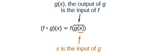
Figure 2
In general, [latex]f\circ g[/latex] and [latex]g\circ f[/latex] are different functions. In other words, in many cases [latex]f\left(g\left(x\right)\right)\ne g\left(f\left(x\right)\right)[/latex] for all [latex]x[/latex]. We will also see that sometimes two functions can be composed only in one specific order.
For example, if [latex]f\left(x\right)={x}^{2}[/latex] and [latex]g\left(x\right)=x+2[/latex], then
[latex]\begin{align}f\left(g\left(x\right)\right)&=f\left(x+2\right) \\ &={\left(x+2\right)}^{2} \\ &={x}^{2}+4x+4 \end{align}[/latex]
but
[latex]\begin{align} g\left(f\left(x\right)\right)&=g\left({x}^{2}\right)\\ &={x}^{2}+2 \end{align}[/latex]
These expressions are not equal for all values of [latex]x[/latex], so the two functions are not equal.
Note that the range of the inside function (the first function to be evaluated) needs to be within the domain of the outside function. Less formally, the composition has to make sense in terms of inputs and outputs.
A General Note: Composition of Functions
When the output of one function is used as the input of another, we call the entire operation a composition of functions. For any input [latex]x[/latex] and functions [latex]f[/latex] and [latex]g[/latex], this action defines a composite function, which we write as [latex]f\circ g[/latex] such that
[latex]\left(f\circ g\right)\left(x\right)=f\left(g\left(x\right)\right)[/latex]
The domain of the composite function [latex]f\circ g[/latex] is all [latex]x[/latex] such that [latex]x[/latex] is in the domain of [latex]g[/latex] and [latex]g\left(x\right)[/latex] is in the domain of [latex]f[/latex].
It is important to realize that the product of functions [latex]fg[/latex] is not the same as the function composition [latex]f\left(g\left(x\right)\right)[/latex], because, in general, [latex]f\left(x\right)g\left(x\right)\ne f\left(g\left(x\right)\right)[/latex].
Example 2: Determining whether Composition of Functions is Commutative
Using the functions below, find [latex]f\left(g\left(x\right)\right)[/latex] and [latex]g\left(f\left(x\right)\right)[/latex]. Determine whether the composition of the functions is commutative.
[latex]f\left(x\right)=2x+1[/latex] [latex]g\left(x\right)=3-x[/latex]
Example 3: Interpreting Composite Functions
The function [latex]c\left(s\right)[/latex] gives the number of calories burned completing [latex]s[/latex] sit-ups, and [latex]s\left(t\right)[/latex] gives the number of sit-ups a person can complete in [latex]t[/latex] minutes. Interpret [latex]c\left(s\left(3\right)\right)[/latex].
Example 4: Investigating the Order of Function Composition
Suppose [latex]f\left(x\right)[/latex] gives miles that can be driven in [latex]x[/latex] hours and [latex]g\left(y\right)[/latex] gives the gallons of gas used in driving [latex]y[/latex] miles. Which of these expressions is meaningful: [latex]f\left(g\left(y\right)\right)[/latex] or [latex]g\left(f\left(x\right)\right)?[/latex]
Q & A
Are there any situations where [latex]f\left(g\left(y\right)\right)[/latex] and [latex]g\left(f\left(x\right)\right)[/latex] would both be meaningful or useful expressions?
Yes. For many pure mathematical functions, both compositions make sense, even though they usually produce different new functions. In real-world problems, functions whose inputs and outputs have the same units also may give compositions that are meaningful in either order.
Try It
The gravitational force on a planet a distance r from the sun is given by the function [latex]G\left(r\right)[/latex]. The acceleration of a planet subjected to any force [latex]F[/latex] is given by the function [latex]a\left(F\right)[/latex]. Form a meaningful composition of these two functions, and explain what it means.
Evaluating Composite Functions
Once we compose a new function from two existing functions, we need to be able to evaluate it for any input in its domain. We will do this with specific numerical inputs for functions expressed as tables, graphs, and formulas and with variables as inputs to functions expressed as formulas. In each case, we evaluate the inner function using the starting input and then use the inner function’s output as the input for the outer function.
Evaluating Composite Functions Using Tables
When working with functions given as tables, we read input and output values from the table entries and always work from the inside to the outside. We evaluate the inside function first and then use the output of the inside function as the input to the outside function.
Example 5: Using a Table to Evaluate a Composite Function
Using the table below, evaluate [latex]f\left(g\left(3\right)\right)[/latex] and [latex]g\left(f\left(3\right)\right)[/latex].
| [latex]x[/latex] | [latex]f\left(x\right)[/latex] | [latex]g\left(x\right)[/latex] |
|---|---|---|
| 1 | 6 | 3 |
| 2 | 8 | 5 |
| 3 | 3 | 2 |
| 4 | 1 | 7 |
Try It
Using the table below, evaluate [latex]f\left(g\left(1\right)\right)[/latex] and [latex]g\left(f\left(4\right)\right)[/latex].
| [latex]x[/latex] | [latex]f\left(x\right)[/latex] | [latex]g\left(x\right)[/latex] |
|---|---|---|
| 1 | 6 | 3 |
| 2 | 8 | 5 |
| 3 | 3 | 2 |
| 4 | 1 | 7 |
Try it 4
Evaluating Composite Functions Using Graphs
When we are given individual functions as graphs, the procedure for evaluating composite functions is similar to the process we use for evaluating tables. We read the input and output values, but this time, from the [latex]x\text{-}[/latex] and [latex]y\text{-}[/latex] axes of the graphs.
How To: Given a composite function and graphs of its individual functions, evaluate it using the information provided by the graphs.
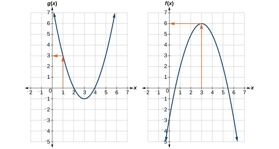
- Locate the given input to the inner function on the [latex]x\text{-}[/latex] axis of its graph.
- Read off the output of the inner function from the [latex]y\text{-}[/latex] axis of its graph.
- Locate the inner function output on the [latex]x\text{-}[/latex] axis of the graph of the outer function.
- Read the output of the outer function from the [latex]y\text{-}[/latex] axis of its graph. This is the output of the composite function.
Example 6: Using a Graph to Evaluate a Composite Function
Using the graphs in Figure 3, evaluate [latex]f\left(g\left(1\right)\right)[/latex].
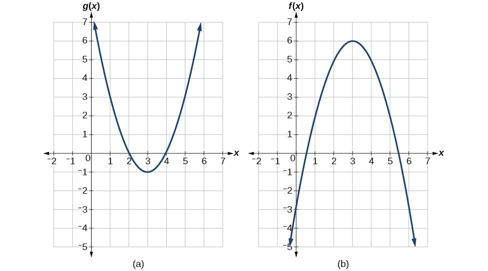
Figure 3
Try It
Using Figure 6, evaluate [latex]g\left(f\left(2\right)\right)[/latex].
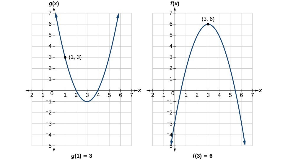
Figure 6
Try It
Evaluating Composite Functions Using Formulas
When evaluating a composite function where we have either created or been given formulas, the rule of working from the inside out remains the same. The input value to the outer function will be the output of the inner function, which may be a numerical value, a variable name, or a more complicated expression.
While we can compose the functions for each individual input value, it is sometimes helpful to find a single formula that will calculate the result of a composition [latex]f\left(g\left(x\right)\right)[/latex]. To do this, we will extend our idea of function evaluation. Recall that, when we evaluate a function like [latex]f\left(t\right)={t}^{2}-t[/latex], we substitute the value inside the parentheses into the formula wherever we see the input variable.
How To: Given a formula for a composite function, evaluate the function.
- Evaluate the inside function using the input value or variable provided.
- Use the resulting output as the input to the outside function.
Example 7: Evaluating a Composition of Functions Expressed as Formulas with a Numerical Input
Given [latex]f\left(t\right)={t}^{2}-{t}[/latex] and [latex]h\left(x\right)=3x+2[/latex], evaluate [latex]f\left(h\left(1\right)\right)[/latex].
Try It
Given [latex]f\left(t\right)={t}^{2}-t[/latex] and [latex]h\left(x\right)=3x+2[/latex], evaluate
A) [latex]h\left(f\left(2\right)\right)[/latex]
B) [latex]h\left(f\left(-2\right)\right)[/latex]
Try It
Finding the Domain of a Composite Function
As we discussed previously, the domain of a composite function such as [latex]f\circ g[/latex] is dependent on the domain of [latex]g[/latex] and the domain of [latex]f[/latex]. It is important to know when we can apply a composite function and when we cannot, that is, to know the domain of a function such as [latex]f\circ g[/latex]. Let us assume we know the domains of the functions [latex]f[/latex] and [latex]g[/latex] separately. If we write the composite function for an input [latex]x[/latex] as [latex]f\left(g\left(x\right)\right)[/latex], we can see right away that [latex]x[/latex] must be a member of the domain of [latex]g[/latex] in order for the expression to be meaningful, because otherwise we cannot complete the inner function evaluation. However, we also see that [latex]g\left(x\right)[/latex] must be a member of the domain of [latex]f[/latex], otherwise the second function evaluation in [latex]f\left(g\left(x\right)\right)[/latex] cannot be completed, and the expression is still undefined. Thus the domain of [latex]f\circ g[/latex] consists of only those inputs in the domain of [latex]g[/latex] that produce outputs from [latex]g[/latex] belonging to the domain of [latex]f[/latex]. Note that the domain of [latex]f[/latex] composed with [latex]g[/latex] is the set of all [latex]x[/latex] such that [latex]x[/latex] is in the domain of [latex]g[/latex] and [latex]g\left(x\right)[/latex] is in the domain of [latex]f[/latex].
A General Note: Domain of a Composite Function
The domain of a composite function [latex]f\left(g\left(x\right)\right)[/latex] is the set of those inputs [latex]x[/latex] in the domain of [latex]g[/latex] for which [latex]g\left(x\right)[/latex] is in the domain of [latex]f[/latex].
How To: Given a function composition [latex]f\left(g\left(x\right)\right)[/latex], determine its domain.
- Find the domain of [latex]g[/latex].
- Find the domain of [latex]f[/latex].
- Find those inputs, [latex]x[/latex], in the domain of [latex]g[/latex] for which [latex]g(x)[/latex] is in the domain of [latex]f[/latex]. That is, exclude those inputs, [latex]x[/latex], from the domain of [latex]g[/latex] for which [latex]g(x)[/latex] is not in the domain of [latex]f[/latex]. The resulting set is the domain of [latex]f\circ g[/latex].
Example 8: Finding the Domain of a Composite Function
Find the domain of
[latex]\left(f\circ g\right)\left(x\right)\text{ where}f\left(x\right)=\frac{5}{x - 1}\text{ and }g\left(x\right)=\frac{4}{3x - 2}[/latex]
Example 9: Finding the Domain of a Composite Function Involving Radicals
Find the domain of
[latex]\left(f\circ g\right)\left(x\right)\text{ where}f\left(x\right)=\sqrt{x+2}\text{ and }g\left(x\right)=\sqrt{3-x}[/latex]
Try It
Find the domain of
[latex]\left(f\circ g\right)\left(x\right)\text{ where}f\left(x\right)=\frac{1}{x - 2}\text{ and }g\left(x\right)=\sqrt{x+4}[/latex]
Try It
Decomposing a Composite Function into its Component Functions
In some cases it is necessary to decompose a complicated function. In other words we can write it as a composition of two simpler functions. There are multiple ways to decompose a composite function, but often one is the most obvious.
Example 10: Decomposing a Function
Write [latex]f\left(x\right)=\sqrt{5-{x}^{2}}[/latex] as the composition of two functions.
Try It
Write [latex]f\left(x\right)=\frac{4}{3-\sqrt{4+{x}^{2}}}[/latex] as the composition of two functions.
Try It
Key Equations
| Composite function | [latex]\left(f\circ g\right)\left(x\right)=f\left(g\left(x\right)\right)[/latex] |
| Average rate of change | [latex]\dfrac{\Delta y}{\Delta x}=\dfrac{f\left({x}_{2}\right)-f\left({x}_{1}\right)}{{x}_{2}-{x}_{1}}[/latex] |
Key Concepts
- A rate of change relates a change in an output quantity to a change in an input quantity. The average rate of change is determined using only the beginning and ending data.
- Identifying points that mark the interval on a graph can be used to find the average rate of change.
- Comparing pairs of input and output values in a table can also be used to find the average rate of change.
- An average rate of change can also be computed by determining the function values at the endpoints of an interval described by a formula.
- The average rate of change can sometimes be determined as an expression.
- A function is increasing where its rate of change is positive and decreasing where its rate of change is negative.
- A local maximum is where a function changes from increasing to decreasing and has an output value larger (more positive or less negative) than output values at neighboring input values.
- A local minimum is where the function changes from decreasing to increasing (as the input increases) and has an output value smaller (more negative or less positive) than output values at neighboring input values.
- Minima and maxima are also called extrema.
- We can find local extrema from a graph.
- When functions are combined, the output of the first (inner) function becomes the input of the second (outer) function.
- The function produced by combining two functions is a composite function.
- The order of function composition must be considered when interpreting the meaning of composite functions.
- A composite function can be evaluated by evaluating the inner function using the given input value and then evaluating the outer function taking as its input the output of the inner function.
- A composite function can be evaluated from a table.
- A composite function can be evaluated from a graph.
- A composite function can be evaluated from a formula.
- The domain of a composite function consists of those inputs in the domain of the inner function that correspond to outputs of the inner function that are in the domain of the outer function.
- Just as functions can be combined to form a composite function, composite functions can be decomposed into simpler functions.
- Functions can often be decomposed in more than one way.
Glossary
- absolute maximum
- the greatest value of a function over an interval
- absolute minimum
- the lowest value of a function over an interval
- average rate of change
- the difference in the output values of a function found for two values of the input divided by the difference between the inputs
- composite function
- the new function formed by function composition, when the output of one function is used as the input of another
- decreasing function
- a function is decreasing in some open interval if [latex]f\left(b\right)
- increasing function
- a function is increasing in some open interval if [latex]f\left(b\right)>f\left(a\right)[/latex] for any two input values [latex]a[/latex] and [latex]b[/latex] in the given interval where [latex]b>a[/latex]
- local extrema
- collectively, all of a function’s local maxima and minima
- local maximum
- a value of the input where a function changes from increasing to decreasing as the input value increases.
- local minimum
- a value of the input where a function changes from decreasing to increasing as the input value increases.
- rate of change
- the change of an output quantity relative to the change of the input quantity
Candela Citations
- Precalculus. Authored by: OpenStax College. Provided by: OpenStax. Located at: http://cnx.org/contents/fd53eae1-fa23-47c7-bb1b-972349835c3c@5.175:1/Preface. License: CC BY: Attribution
- http://www.eia.gov/totalenergy/data/annual/showtext.cfm?t=ptb0524. Accessed 3/5/2014. ↵