
Figure 1. Electron micrograph of E.Coli bacteria (credit: “Mattosaurus,” Wikimedia Commons)
Focus in on a square centimeter of your skin. Look closer. Closer still. If you could look closely enough, you would see hundreds of thousands of microscopic organisms. They are bacteria, and they are not only on your skin, but in your mouth, nose, and even your intestines. In fact, the bacterial cells in your body at any given moment outnumber your own cells. But that is no reason to feel bad about yourself. While some bacteria can cause illness, many are healthy and even essential to the body.
Bacteria commonly reproduce through a process called binary fission, during which one bacterial cell splits into two. When conditions are right, bacteria can reproduce very quickly. Unlike humans and other complex organisms, the time required to form a new generation of bacteria is often a matter of minutes or hours, as opposed to days or years.[1]
For simplicity’s sake, suppose we begin with a culture of one bacterial cell that can divide every hour. The table below shows the number of bacterial cells at the end of each subsequent hour. We see that the single bacterial cell leads to over one thousand bacterial cells in just ten hours! And if we were to extrapolate the table to twenty-four hours, we would have over 16 million!
| Hour | 0 | 1 | 2 | 3 | 4 | 5 | 6 | 7 | 8 | 9 | 10 |
| Bacteria | 1 | 2 | 4 | 8 | 16 | 32 | 64 | 128 | 256 | 512 | 1024 |
Exponential Functions
In this chapter, we will explore exponential functions, which can be used for, among other things, modeling growth patterns such as those found in bacteria. We will also investigate logarithmic functions, which are closely related to exponential functions. Both types of functions have numerous real-world applications when it comes to modeling and interpreting data.
Learning Outcomes
- Evaluate exponential functions.
- Find the equation of an exponential function.
- Use compound interest formulas.
- Evaluate exponential functions with base e.
- Graph exponential functions.
- Graph exponential functions using transformations.
India is the second most populous country in the world with a population of about 1.25 billion people in 2013. The population is growing at a rate of about 1.2% each year.[2] If this rate continues, the population of India will exceed China’s population by the year 2031. When populations grow rapidly, we often say that the growth is “exponential,” meaning that something is growing very rapidly. To a mathematician, however, the term exponential growth has a very specific meaning. In this section, we will take a look at exponential functions, which model this kind of rapid growth.
Evaluate Exponential Functions
Recall that the base of an exponential function must be a positive real number other than 1. Why do we limit the base b to positive values? To ensure that the outputs will be real numbers. Observe what happens if the base is not positive:
- Let b = –9 and [latex]x=\frac{1}{2}[/latex]. Then [latex]f\left(x\right)=f\left(\frac{1}{2}\right)={\left(-9\right)}^{\frac{1}{2}}=\sqrt{-9}[/latex], which is not a real number.
Why do we limit the base to positive values other than 1? Because base 1 results in the constant function. Observe what happens if the base is 1:
- Let b = 1. Then [latex]f\left(x\right)={1}^{x}=1[/latex] for any value of x.
To evaluate an exponential function with the form [latex]f\left(x\right)={b}^{x}[/latex], we simply substitute x with the given value, and calculate the resulting power. For example:
Let [latex]f\left(x\right)={2}^{x}[/latex]. What is [latex]f\left(3\right)[/latex]?
To evaluate an exponential function with a form other than the basic form, it is important to follow the order of operations. For example:
Let [latex]f\left(x\right)=30{\left(2\right)}^{x}[/latex]. What is [latex]f\left(3\right)[/latex]?
Note that if the order of operations were not followed, the result would be incorrect:
[latex]f\left(3\right)=30{\left(2\right)}^{3}\ne {60}^{3}=216,000[/latex]
Example 1: Evaluating Exponential Functions
Let [latex]f\left(x\right)=5{\left(3\right)}^{x+1}[/latex]. Evaluate [latex]f\left(2\right)[/latex] without using a calculator.
Try It
Let [latex]f\left(x\right)=8{\left(1.2\right)}^{x - 5}[/latex]. Evaluate [latex]f\left(3\right)[/latex] using a calculator. Round to four decimal places.
Because the output of exponential functions increases very rapidly, the term “exponential growth” is often used in everyday language to describe anything that grows or increases rapidly. However, exponential growth can be defined more precisely in a mathematical sense. If the growth rate is proportional to the amount present, the function models exponential growth.
A General Note: Exponential Growth
A function that models exponential growth grows by a rate proportional to the amount present. For any real number x and any positive real numbers a and b such that [latex]b\ne 1[/latex], an exponential growth function has the form
where
- a is the initial or starting value of the function.
- b is the growth factor or growth multiplier per unit x.
In more general terms, we have an exponential function, in which a constant base is raised to a variable exponent. To differentiate between linear and exponential functions, let’s consider two companies, A and B. Company A has 100 stores and expands by opening 50 new stores a year, so its growth can be represented by the function [latex]A\left(x\right)=100+50x[/latex]. Company B has 100 stores and expands by increasing the number of stores by 50% each year, so its growth can be represented by the function [latex]B\left(x\right)=100{\left(1+0.5\right)}^{x}[/latex].
A few years of growth for these companies are illustrated below.
| Year, x | Stores, Company A | Stores, Company B |
|---|---|---|
| 0 | 100 + 50(0) = 100 | 100(1 + 0.5)0 = 100 |
| 1 | 100 + 50(1) = 150 | 100(1 + 0.5)1 = 150 |
| 2 | 100 + 50(2) = 200 | 100(1 + 0.5)2 = 225 |
| 3 | 100 + 50(3) = 250 | 100(1 + 0.5)3 = 337.5 |
| x | A(x) = 100 + 50x | B(x) = 100(1 + 0.5)x |
The graphs comparing the number of stores for each company over a five-year period are shown in below. We can see that, with exponential growth, the number of stores increases much more rapidly than with linear growth.
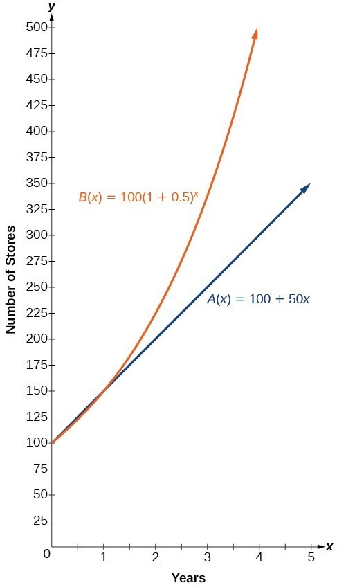
Figure 2. The graph shows the numbers of stores Companies A and B opened over a five-year period.
Notice that the domain for both functions is [latex]\left[0,\infty \right)[/latex], and the range for both functions is [latex]\left[100,\infty \right)[/latex]. After year 1, Company B always has more stores than Company A.
Now we will turn our attention to the function representing the number of stores for Company B, [latex]B\left(x\right)=100{\left(1+0.5\right)}^{x}[/latex]. In this exponential function, 100 represents the initial number of stores, 0.50 represents the growth rate, and [latex]1+0.5=1.5[/latex] represents the growth factor. Generalizing further, we can write this function as [latex]B\left(x\right)=100{\left(1.5\right)}^{x}[/latex], where 100 is the initial value, 1.5 is called the base, and x is called the exponent.
Example 2: Evaluating a Real-World Exponential Model
At the beginning of this section, we learned that the population of India was about 1.25 billion in the year 2013, with an annual growth rate of about 1.2%. This situation is represented by the growth function [latex]P\left(t\right)=1.25{\left(1.012\right)}^{t}[/latex], where t is the number of years since 2013. To the nearest thousandth, what will the population of India be in 2031?
Try It
The population of China was about 1.39 billion in the year 2013, with an annual growth rate of about 0.6%. This situation is represented by the growth function [latex]P\left(t\right)=1.39{\left(1.006\right)}^{t}[/latex], where t is the number of years since 2013. To the nearest thousandth, what will the population of China be for the year 2031? How does this compare to the population prediction we made for India in Example 2?
Find the Equation of an Exponential Function
In the previous examples, we were given an exponential function, which we then evaluated for a given input. Sometimes we are given information about an exponential function without knowing the function explicitly. We must use the information to first write the form of the function, then determine the constants a and b, and evaluate the function.
How To: Given two data points, write an exponential model.
- If one of the data points has the form [latex]\left(0,a\right)[/latex], then a is the initial value. Using a, substitute the second point into the equation [latex]f\left(x\right)=a{\left(b\right)}^{x}[/latex], and solve for b.
- If neither of the data points have the form [latex]\left(0,a\right)[/latex], substitute both points into two equations with the form [latex]f\left(x\right)=a{\left(b\right)}^{x}[/latex]. Solve the resulting system of two equations in two unknowns to find a and b.
- Using the a and b found in the steps above, write the exponential function in the form [latex]f\left(x\right)=a{\left(b\right)}^{x}[/latex].
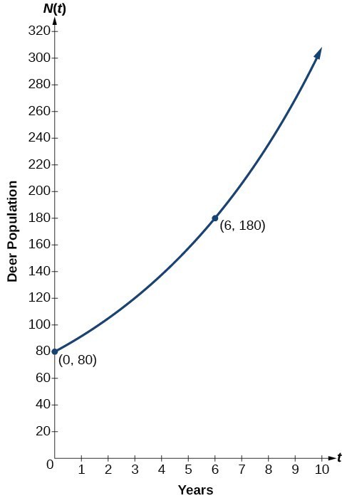
Example 3: Writing an Exponential Model When the Initial Value Is Known
In 2006, 80 deer were introduced into a wildlife refuge. By 2012, the population had grown to 180 deer. The population was growing exponentially. Write an algebraic function N(t) representing the population N of deer over time t.
Try It
A wolf population is growing exponentially. In 2011, 129 wolves were counted. By 2013 the population had reached 236 wolves. What two points can be used to derive an exponential equation modeling this situation? Write the equation representing the population N of wolves over time t.
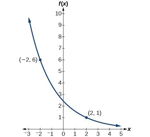
Example 4: Writing an Exponential Model When the Initial Value is Not Known
Find an exponential function that passes through the points [latex]\left(-2,6\right)[/latex] and [latex]\left(2,1\right)[/latex].
Try It
Given the two points [latex]\left(1,3\right)[/latex] and [latex]\left(2,4.5\right)[/latex], find the equation of the exponential function that passes through these two points.
Try It
Q & A
Do two points always determine a unique exponential function?
Yes, provided the two points are either both above the x-axis or both below the x-axis and have different x-coordinates. But keep in mind that we also need to know that the graph is, in fact, an exponential function. Not every graph that looks exponential really is exponential. We need to know the graph is based on a model that shows the same percent growth with each unit increase in x, which in many real world cases involves time.
How To: Given the graph of an exponential function, write its equation.
- First, identify two points on the graph. Choose the y-intercept as one of the two points whenever possible. Try to choose points that are as far apart as possible to reduce round-off error.
- If one of the data points is the y-intercept [latex]\left(0,a\right)[/latex] , then a is the initial value. Using a, substitute the second point into the equation [latex]f\left(x\right)=a{\left(b\right)}^{x}[/latex], and solve for b.
- If neither of the data points have the form [latex]\left(0,a\right)[/latex], substitute both points into two equations with the form [latex]f\left(x\right)=a{\left(b\right)}^{x}[/latex]. Solve the resulting system of two equations in two unknowns to find a and b.
- Write the exponential function, [latex]f\left(x\right)=a{\left(b\right)}^{x}[/latex].
Example 5: Writing an Exponential Function Given Its Graph
Find an equation for the exponential function graphed in Figure 5.
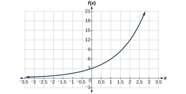
Figure 5
Try It
Find an equation for the exponential function graphed in Figure 6.
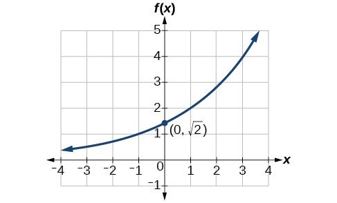
Figure 6
Try It
How To: Given two points on the curve of an exponential function, use a graphing calculator to find the equation.
- Press [STAT].
- Clear any existing entries in columns L1 or L2.
- In L1, enter the x-coordinates given.
- In L2, enter the corresponding y-coordinates.
- Press [STAT] again. Cursor right to CALC, scroll down to ExpReg (Exponential Regression), and press [ENTER].
- The screen displays the values of a and b in the exponential equation [latex]y=a\cdot {b}^{x}[/latex].
Example 6: Using a Graphing Calculator to Find an Exponential Function
Use a graphing calculator to find the exponential equation that includes the points [latex]\left(2,24.8\right)[/latex] and [latex]\left(5,198.4\right)[/latex].
Try It
Use a graphing calculator to find the exponential function that includes the points (3, 75.98) and (6, 481.07).
Use Compound Interest Formulas
Savings instruments in which earnings are continually reinvested, such as mutual funds and retirement accounts, use compound interest. The term compounding refers to interest earned not only on the original value, but on the accumulated value of the account.
The annual percentage rate (APR) of an account, also called the nominal rate, is the yearly interest rate earned by an investment account. The term nominal is used when the compounding occurs a number of times other than once per year. In fact, when interest is compounded more than once a year, the effective interest rate ends up being greater than the nominal rate! This is a powerful tool for investing.
We can calculate the compound interest using the compound interest formula, which is an exponential function of the variables time t, principal P, APR r, and number of compounding periods in a year n:
For example, observe the table below, which shows the result of investing $1,000 at 10% for one year. Notice how the value of the account increases as the compounding frequency increases.
| Frequency | Value after 1 year |
|---|---|
| Annually | $1100 |
| Semiannually | $1102.50 |
| Quarterly | $1103.81 |
| Monthly | $1104.71 |
| Daily | $1105.16 |
A General Note: The Compound Interest Formula
Compound interest can be calculated using the formula
where
- A(t) is the account value,
- t is measured in years,
- P is the starting amount of the account, often called the principal, or more generally present value,
- r is the annual percentage rate (APR) expressed as a decimal, and
- n is the number of compounding periods in one year.
Example 7: Calculating Compound Interest
If we invest $3,000 in an investment account paying 3% interest compounded quarterly, how much will the account be worth in 10 years?
Try It
An initial investment of $100,000 at 12% interest is compounded weekly (use 52 weeks in a year). What will the investment be worth in 30 years?
Example 8: Using the Compound Interest Formula to Solve for the Principal
A 529 Plan is a college-savings plan that allows relatives to invest money to pay for a child’s future college tuition; the account grows tax-free. Lily wants to set up a 529 account for her new granddaughter and wants the account to grow to $40,000 over 18 years. She believes the account will earn 6% compounded semi-annually (twice a year). To the nearest dollar, how much will Lily need to invest in the account now?
Try It
Refer to Example 8. To the nearest dollar, how much would Lily need to invest if the account is compounded quarterly?
Try It
Evaluate exponential functions with base e
As we saw earlier, the amount earned on an account increases as the compounding frequency increases. The table below shows that the increase from annual to semi-annual compounding is larger than the increase from monthly to daily compounding. This might lead us to ask whether this pattern will continue.
Examine the value of $1 invested at 100% interest for 1 year, compounded at various frequencies.
| Frequency | [latex]A\left(t\right)={\left(1+\frac{1}{n}\right)}^{n}[/latex] | Value |
|---|---|---|
| Annually | [latex]{\left(1+\frac{1}{1}\right)}^{1}[/latex] | $2 |
| Semiannually | [latex]{\left(1+\frac{1}{2}\right)}^{2}[/latex] | $2.25 |
| Quarterly | [latex]{\left(1+\frac{1}{4}\right)}^{4}[/latex] | $2.441406 |
| Monthly | [latex]{\left(1+\frac{1}{12}\right)}^{12}[/latex] | $2.613035 |
| Daily | [latex]{\left(1+\frac{1}{365}\right)}^{365}[/latex] | $2.714567 |
| Hourly | [latex]{\left(1+\frac{1}{\text{8766}}\right)}^{\text{8766}}[/latex] | $2.718127 |
| Once per minute | [latex]{\left(1+\frac{1}{\text{525960}}\right)}^{\text{525960}}[/latex] | $2.718279 |
| Once per second | [latex]{\left(1+\frac{1}{31557600}\right)}^{31557600}[/latex] | $2.718282 |
These values appear to be approaching a limit as n increases without bound. In fact, as n gets larger and larger, the expression [latex]{\left(1+\frac{1}{n}\right)}^{n}[/latex] approaches a number used so frequently in mathematics that it has its own name: the letter [latex]e[/latex]. This value is an irrational number, which means that its decimal expansion goes on forever without repeating. Its approximation to six decimal places is shown below.
A General Note: The Number e
The letter e represents the irrational number
[latex]{\left(1+\frac{1}{n}\right)}^{n},\text{as}n\text{increases without bound}[/latex]
The letter e is used as a base for many real-world exponential models. To work with base e, we use the approximation, [latex]e\approx 2.718282[/latex]. The constant was named by the Swiss mathematician Leonhard Euler (1707–1783) who first investigated and discovered many of its properties.
Example 9: Using a Calculator to Find Powers of e
Calculate [latex]{e}^{3.14}[/latex]. Round to five decimal places.
Try It
Use a calculator to find [latex]{e}^{-0.5}[/latex]. Round to five decimal places.
Investigating Continuous Growth
So far we have worked with rational bases for exponential functions. For most real-world phenomena, however, e is used as the base for exponential functions. Exponential models that use e as the base are called continuous growth or decay models. We see these models in finance, computer science, and most of the sciences, such as physics, toxicology, and fluid dynamics.
A General Note: The Continuous Growth/Decay Formula
For all real numbers t, and all positive numbers a and r, continuous growth or decay is represented by the formula
where
- a is the initial value,
- r is the continuous growth rate per unit time,
- and t is the elapsed time.
If r > 0, then the formula represents continuous growth. If r < 0, then the formula represents continuous decay.
For business applications, the continuous growth formula is called the continuous compounding formula and takes the form
where
- P is the principal or the initial invested,
- r is the growth or interest rate per unit time,
- and t is the period or term of the investment.
How To: Given the initial value, rate of growth or decay, and time t, solve a continuous growth or decay function.
- Use the information in the problem to determine a, the initial value of the function.
- Use the information in the problem to determine the growth rate r.
- If the problem refers to continuous growth, then r > 0.
- If the problem refers to continuous decay, then r < 0.
- Use the information in the problem to determine the time t.
- Substitute the given information into the continuous growth formula and solve for A(t).
Example 10: Calculating Continuous Growth
A person invested $1,000 in an account earning a nominal 10% per year compounded continuously. How much was in the account at the end of one year?
Try It
A person invests $100,000 at a nominal 12% interest per year compounded continuously. What will be the value of the investment in 30 years?
Example 11: Calculating Continuous Decay
Radon-222 decays at a continuous rate of 17.3% per day. How much will 100 mg of Radon-222 decay to in 3 days?
Try It
Using the data in Example 9, how much radon-222 will remain after one year?
Try It
Working with an equation that describes a real-world situation gives us a method for making predictions. Most of the time, however, the equation itself is not enough. We learn a lot about things by seeing their pictorial representations, and that is exactly why graphing exponential equations is a powerful tool. It gives us another layer of insight for predicting future events.
Graph exponential functions
Before we begin graphing, it is helpful to review the behavior of exponential growth. Recall the table of values for a function of the form [latex]f\left(x\right)={b}^{x}[/latex] whose base is greater than one. We’ll use the function [latex]f\left(x\right)={2}^{x}[/latex]. Observe how the output values in the table below change as the input increases by 1.
| x | –3 | –2 | –1 | 0 | 1 | 2 | 3 |
| [latex]f\left(x\right)={2}^{x}[/latex] | [latex]\frac{1}{8}[/latex] | [latex]\frac{1}{4}[/latex] | [latex]\frac{1}{2}[/latex] | 1 | 2 | 4 | 8 |
Each output value is the product of the previous output and the base, 2. We call the base 2 the constant ratio. In fact, for any exponential function with the form [latex]f\left(x\right)=a{b}^{x}[/latex], b is the constant ratio of the function. This means that as the input increases by 1, the output value will be the product of the base and the previous output, regardless of the value of a.
Notice from the table that
- the output values are positive for all values of x;
- as x increases, the output values increase without bound; and
- as x decreases, the output values grow smaller, approaching zero.
Figure 1 shows the exponential growth function [latex]f\left(x\right)={2}^{x}[/latex].
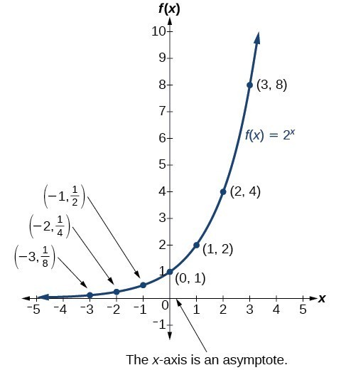
Figure 1. Notice that the graph gets close to the x-axis, but never touches it.
The domain of [latex]f\left(x\right)={2}^{x}[/latex] is all real numbers, the range is [latex]\left(0,\infty \right)[/latex], and the horizontal asymptote is [latex]y=0[/latex].
To get a sense of the behavior of exponential decay, we can create a table of values for a function of the form [latex]f\left(x\right)={b}^{x}[/latex] whose base is between zero and one. We’ll use the function [latex]g\left(x\right)={\left(\frac{1}{2}\right)}^{x}[/latex]. Observe how the output values in the table below change as the input increases by 1.
| x | –3 | –2 | –1 | 0 | 1 | 2 | 3 |
| [latex]g\left(x\right)=\left(\frac{1}{2}\right)^{x}[/latex] | 8 | 4 | 2 | 1 | [latex]\frac{1}{2}[/latex] | [latex]\frac{1}{4}[/latex] | [latex]\frac{1}{8}[/latex] |
Again, because the input is increasing by 1, each output value is the product of the previous output and the base, or constant ratio [latex]\frac{1}{2}[/latex].
Notice from the table that
- the output values are positive for all values of x;
- as x increases, the output values grow smaller, approaching zero; and
- as x decreases, the output values grow without bound.
The graph shows the exponential decay function, [latex]g\left(x\right)={\left(\frac{1}{2}\right)}^{x}[/latex].
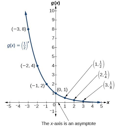
Figure 2. The domain of [latex]g\left(x\right)={\left(\frac{1}{2}\right)}^{x}[/latex] is all real numbers, the range is [latex]\left(0,\infty \right)[/latex], and the horizontal asymptote is [latex]y=0[/latex].
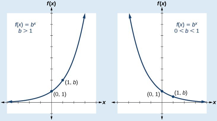
A General Note: Characteristics of the Graph of the Parent Function f(x) = bx
An exponential function with the form [latex]f\left(x\right)={b}^{x}[/latex], [latex]b>0[/latex], [latex]b\ne 1[/latex], has these characteristics:
- one-to-one function
- horizontal asymptote: [latex]y=0[/latex]
- domain: [latex]\left(-\infty , \infty \right)[/latex]
- range: [latex]\left(0,\infty \right)[/latex]
- x-intercept: none
- y-intercept: [latex]\left(0,1\right)[/latex]
- increasing if [latex]b>1[/latex]
- decreasing if [latex]b<1[/latex]
Compare the graphs of exponential growth and decay functions.
How To: Given an exponential function of the form [latex]f\left(x\right)={b}^{x}[/latex], graph the function.
- Create a table of points.
- Plot at least 3 point from the table, including the y-intercept [latex]\left(0,1\right)[/latex].
- Draw a smooth curve through the points.
- State the domain, [latex]\left(-\infty ,\infty \right)[/latex], the range, [latex]\left(0,\infty \right)[/latex], and the horizontal asymptote, [latex]y=0[/latex].
Example 1: Sketching the Graph of an Exponential Function of the Form f(x) = bx
Sketch a graph of [latex]f\left(x\right)={0.25}^{x}[/latex]. State the domain, range, and asymptote.
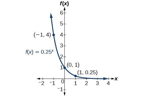
Try It
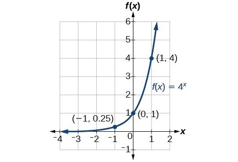
Sketch the graph of [latex]f\left(x\right)={4}^{x}[/latex]. State the domain, range, and asymptote.
Graph exponential functions using transformations
Transformations of exponential graphs behave similarly to those of other functions. Just as with other parent functions, we can apply the four types of transformations—shifts, reflections, stretches, and compressions—to the parent function [latex]f\left(x\right)={b}^{x}[/latex] without loss of shape. For instance, just as the quadratic function maintains its parabolic shape when shifted, reflected, stretched, or compressed, the exponential function also maintains its general shape regardless of the transformations applied.
Graphing a Vertical Shift
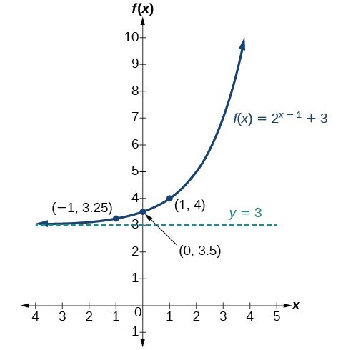
The first transformation occurs when we add a constant d to the parent function [latex]f\left(x\right)={b}^{x}[/latex], giving us a vertical shift d units in the same direction as the sign. For example, if we begin by graphing a parent function, [latex]f\left(x\right)={2}^{x}[/latex], we can then graph two vertical shifts alongside it, using [latex]d=3[/latex]: the upward shift, [latex]g\left(x\right)={2}^{x}+3[/latex] and the downward shift, [latex]h\left(x\right)={2}^{x}-3[/latex]. Both vertical shifts are shown in Figure 5.
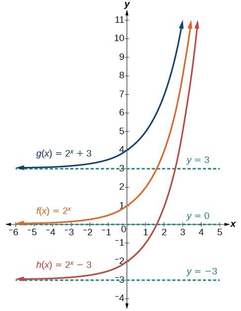
Figure 5
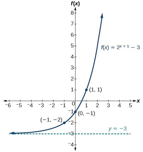
Observe the results of shifting [latex]f\left(x\right)={2}^{x}[/latex] vertically:
- The domain, [latex]\left(-\infty ,\infty \right)[/latex] remains unchanged.
- When the function is shifted up 3 units to [latex]g\left(x\right)={2}^{x}+3[/latex]:
- The y-intercept shifts up 3 units to [latex]\left(0,4\right)[/latex].
- The asymptote shifts up 3 units to [latex]y=3[/latex].
- The range becomes [latex]\left(3,\infty \right)[/latex].
- When the function is shifted down 3 units to [latex]h\left(x\right)={2}^{x}-3[/latex]:
- The y-intercept shifts down 3 units to [latex]\left(0,-2\right)[/latex].
- The asymptote also shifts down 3 units to [latex]y=-3[/latex].
- The range becomes [latex]\left(-3,\infty \right)[/latex].
Graphing a Horizontal Shift
The next transformation occurs when we add a constant c to the input of the parent function [latex]f\left(x\right)={b}^{x}[/latex], giving us a horizontal shift c units in the opposite direction of the sign. For example, if we begin by graphing the parent function [latex]f\left(x\right)={2}^{x}[/latex], we can then graph two horizontal shifts alongside it, using [latex]c=3[/latex]: the shift left, [latex]g\left(x\right)={2}^{x+3}[/latex], and the shift right, [latex]h\left(x\right)={2}^{x - 3}[/latex]. Both horizontal shifts are shown in Figure 6.
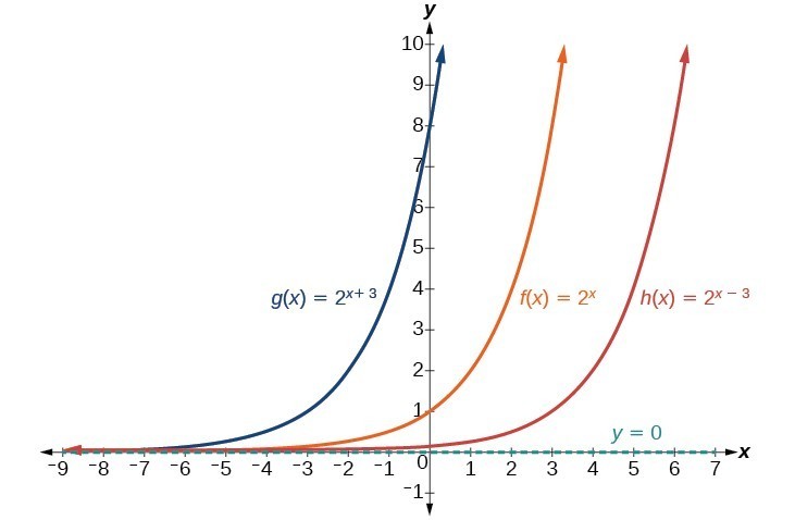
Figure 6
Observe the results of shifting [latex]f\left(x\right)={2}^{x}[/latex] horizontally:
- The domain, [latex]\left(-\infty ,\infty \right)[/latex], remains unchanged.
- The asymptote, [latex]y=0[/latex], remains unchanged.
- The y-intercept shifts such that:
- When the function is shifted left 3 units to [latex]g\left(x\right)={2}^{x+3}[/latex], the y-intercept becomes [latex]\left(0,8\right)[/latex]. This is because [latex]{2}^{x+3}=\left(8\right){2}^{x}[/latex], so the initial value of the function is 8.
- When the function is shifted right 3 units to [latex]h\left(x\right)={2}^{x - 3}[/latex], the y-intercept becomes [latex]\left(0,\frac{1}{8}\right)[/latex]. Again, see that [latex]{2}^{x - 3}=\left(\frac{1}{8}\right){2}^{x}[/latex], so the initial value of the function is [latex]\frac{1}{8}[/latex].
A General Note: Shifts of the Parent Function [latex]f\left(x\right)={b}^{x}[/latex]
For any constants c and d, the function [latex]f\left(x\right)={b}^{x+c}+d[/latex] shifts the parent function [latex]f\left(x\right)={b}^{x}[/latex]
- vertically d units, in the same direction of the sign of d.
- horizontally c units, in the opposite direction of the sign of c.
- The y-intercept becomes [latex]\left(0,{b}^{c}+d\right)[/latex].
- The horizontal asymptote becomes y = d.
- The range becomes [latex]\left(d,\infty \right)[/latex].
- The domain, [latex]\left(-\infty ,\infty \right)[/latex], remains unchanged.
How To: Given an exponential function with the form [latex]f\left(x\right)={b}^{x+c}+d[/latex], graph the translation.
- Draw the horizontal asymptote y = d.
- Identify the shift as [latex]\left(-c,d\right)[/latex]. Shift the graph of [latex]f\left(x\right)={b}^{x}[/latex] left c units if c is positive, and right [latex]c[/latex] units if c is negative.
- Shift the graph of [latex]f\left(x\right)={b}^{x}[/latex] up d units if d is positive, and down d units if d is negative.
- State the domain, [latex]\left(-\infty ,\infty \right)[/latex], the range, [latex]\left(d,\infty \right)[/latex], and the horizontal asymptote [latex]y=d[/latex].
Example 2: Graphing a Shift of an Exponential Function
Graph [latex]f\left(x\right)={2}^{x+1}-3[/latex]. State the domain, range, and asymptote.
Try It
Graph [latex]f\left(x\right)={2}^{x - 1}+3[/latex]. State domain, range, and asymptote.
Try It
How To: Given an equation of the form [latex]f\left(x\right)={b}^{x+c}+d[/latex] for [latex]x[/latex], use a graphing calculator to approximate the solution.
- Press [Y=]. Enter the given exponential equation in the line headed “Y1=.”
- Enter the given value for [latex]f\left(x\right)[/latex] in the line headed “Y2=.”
- Press [WINDOW]. Adjust the y-axis so that it includes the value entered for “Y2=.”
- Press [GRAPH] to observe the graph of the exponential function along with the line for the specified value of [latex]f\left(x\right)[/latex].
- To find the value of x, we compute the point of intersection. Press [2ND] then [CALC]. Select “intersect” and press [ENTER] three times. The point of intersection gives the value of x for the indicated value of the function.
Example 3: Approximating the Solution of an Exponential Equation
Solve [latex]42=1.2{\left(5\right)}^{x}+2.8[/latex] graphically. Round to the nearest thousandth.
Try It
Solve [latex]4=7.85{\left(1.15\right)}^{x}-2.27[/latex] graphically. Round to the nearest thousandth.
Graphing a Stretch or Compression
While horizontal and vertical shifts involve adding constants to the input or to the function itself, a stretch or compression occurs when we multiply the parent function [latex]f\left(x\right)={b}^{x}[/latex] by a constant [latex]|a|>0[/latex]. For example, if we begin by graphing the parent function [latex]f\left(x\right)={2}^{x}[/latex], we can then graph the stretch, using [latex]a=3[/latex], to get [latex]g\left(x\right)=3{\left(2\right)}^{x}[/latex] as shown on the left in Figure 8, and the compression, using [latex]a=\frac{1}{3}[/latex], to get [latex]h\left(x\right)=\frac{1}{3}{\left(2\right)}^{x}[/latex] as shown on the right in Figure 8.
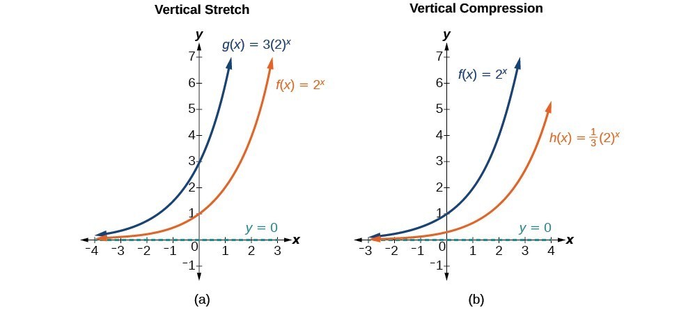
Figure 8. (a) [latex]g\left(x\right)=3{\left(2\right)}^{x}[/latex] stretches the graph of [latex]f\left(x\right)={2}^{x}[/latex] vertically by a factor of 3. (b) [latex]h\left(x\right)=\frac{1}{3}{\left(2\right)}^{x}[/latex] compresses the graph of [latex]f\left(x\right)={2}^{x}[/latex] vertically by a factor of [latex]\frac{1}{3}[/latex].
A General Note: Stretches and Compressions of the Parent Function f(x) = bx
For any factor a > 0, the function [latex]f\left(x\right)=a{\left(b\right)}^{x}[/latex]
- is stretched vertically by a factor of a if [latex]|a|>1[/latex].
- is compressed vertically by a factor of a if [latex]|a|<1[/latex].
- has a y-intercept of [latex]\left(0,a\right)[/latex].
- has a horizontal asymptote at [latex]y=0[/latex], a range of [latex]\left(0,\infty \right)[/latex], and a domain of [latex]\left(-\infty ,\infty \right)[/latex], which are unchanged from the parent function.
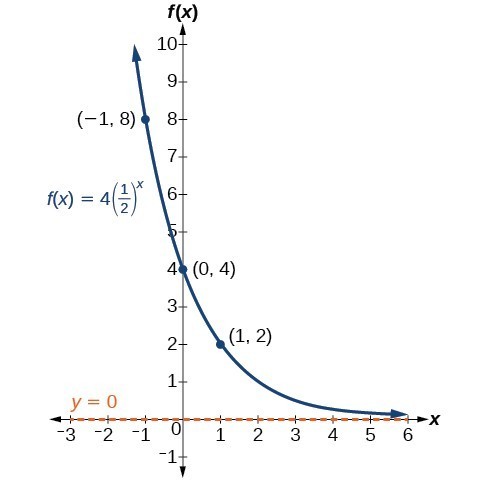
Example 4: Graphing the Stretch of an Exponential Function
Sketch a graph of [latex]f\left(x\right)=4{\left(\frac{1}{2}\right)}^{x}[/latex]. State the domain, range, and asymptote.
Try It
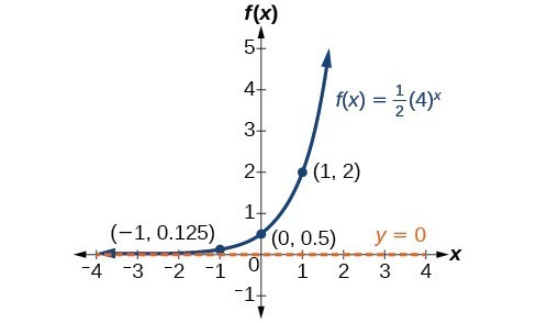
Sketch the graph of [latex]f\left(x\right)=\frac{1}{2}{\left(4\right)}^{x}[/latex]. State the domain, range, and asymptote.
Try It
Graphing Reflections
In addition to shifting, compressing, and stretching a graph, we can also reflect it about the x-axis or the y-axis. When we multiply the parent function [latex]f\left(x\right)={b}^{x}[/latex] by –1, we get a reflection about the x-axis. When we multiply the input by –1, we get a reflection about the y-axis. For example, if we begin by graphing the parent function [latex]f\left(x\right)={2}^{x}[/latex], we can then graph the two reflections alongside it. The reflection about the x-axis, [latex]g\left(x\right)={-2}^{x}[/latex], is shown on the left side, and the reflection about the y-axis [latex]h\left(x\right)={2}^{-x}[/latex], is shown on the right side.
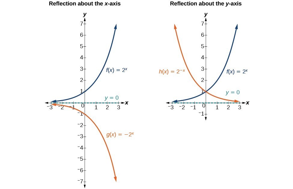
(a) [latex]g\left(x\right)=-{2}^{x}[/latex] reflects the graph of [latex]f\left(x\right)={2}^{x}[/latex] about the x-axis.
(b) [latex]g\left(x\right)={2}^{-x}[/latex] reflects the graph of [latex]f\left(x\right)={2}^{x}[/latex] about the y-axis.
A General Note: Reflections of the Parent Function f(x) = bx
The function [latex]f\left(x\right)=-{b}^{x}[/latex]
- reflects the parent function [latex]f\left(x\right)={b}^{x}[/latex] about the x-axis.
- has a y-intercept of [latex]\left(0,-1\right)[/latex].
- has a range of [latex]\left(-\infty ,0\right)[/latex]
- has a horizontal asymptote at [latex]y=0[/latex] and domain of [latex]\left(-\infty ,\infty \right)[/latex], which are unchanged from the parent function.
The function [latex]f\left(x\right)={b}^{-x}[/latex]
- reflects the parent function [latex]f\left(x\right)={b}^{x}[/latex] about the y-axis.
- has a y-intercept of [latex]\left(0,1\right)[/latex], a horizontal asymptote at [latex]y=0[/latex], a range of [latex]\left(0,\infty \right)[/latex], and a domain of [latex]\left(-\infty ,\infty \right)[/latex], which are unchanged from the parent function.
Example 5: Writing and Graphing the Reflection of an Exponential Function
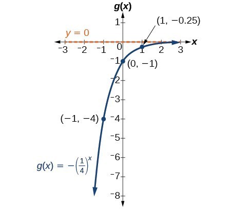
Find and graph the equation for a function, [latex]g\left(x\right)[/latex], that reflects [latex]f\left(x\right)={\left(\frac{1}{4}\right)}^{x}[/latex] about the x-axis. State its domain, range, and asymptote.
Try It
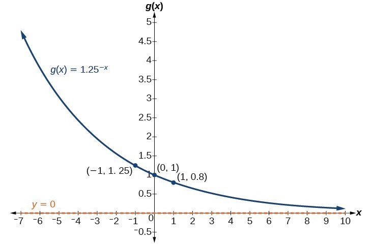
Find and graph the equation for a function, [latex]g\left(x\right)[/latex], that reflects [latex]f\left(x\right)={1.25}^{x}[/latex] about the y-axis. State its domain, range, and asymptote.
Try It
Summarizing Translations of the Exponential Function
Now that we have worked with each type of translation for the exponential function, we can summarize them to arrive at the general equation for translating exponential functions.
| Translations of the Parent Function [latex]f\left(x\right)={b}^{x}[/latex] | |
|---|---|
| Translation | Form |
Shift
|
[latex]f\left(x\right)={b}^{x+c}+d[/latex] |
Stretch and Compress
|
[latex]f\left(x\right)=a{b}^{x}[/latex] |
| Reflect about the x-axis | [latex]f\left(x\right)=-{b}^{x}[/latex] |
| Reflect about the y-axis | [latex]f\left(x\right)={b}^{-x}={\left(\frac{1}{b}\right)}^{x}[/latex] |
| General equation for all translations | [latex]f\left(x\right)=a{b}^{x+c}+d[/latex] |
A General Note: Translations of Exponential Functions
A translation of an exponential function has the form
Where the parent function, [latex]y={b}^{x}[/latex], [latex]b>1[/latex], is
- shifted horizontally c units to the left.
- stretched vertically by a factor of |a| if |a| > 0.
- compressed vertically by a factor of |a| if 0 < |a| < 1.
- shifted vertically d units.
- reflected about the x-axis when a < 0.
Note the order of the shifts, transformations, and reflections follow the order of operations.
Example 6: Writing a Function from a Description
Write the equation for the function described below. Give the horizontal asymptote, the domain, and the range.
[latex]f\left(x\right)={e}^{x}[/latex] is vertically stretched by a factor of 2, reflected across the y-axis, and then shifted up 4 units.
Try It
Write the equation for function described below. Give the horizontal asymptote, the domain, and the range.
[latex]f\left(x\right)={e}^{x}[/latex] is compressed vertically by a factor of [latex]\frac{1}{3}[/latex], reflected across the x-axis and then shifted down 2 units.
Key Equations
| definition of the exponential function | [latex]f\left(x\right)={b}^{x}\text{, where }b>0, b\ne 1[/latex] |
| definition of exponential growth | [latex]f\left(x\right)=a{b}^{x},\text{ where }a>0,b>0,b\ne 1[/latex] |
| compound interest formula | [latex]\begin{cases}A\left(t\right)=P{\left(1+\frac{r}{n}\right)}^{nt} ,\text{ where}\hfill \\ A\left(t\right)\text{ is the account value at time }t\hfill \\ t\text{ is the number of years}\hfill \\ P\text{ is the initial investment, often called the principal}\hfill \\ r\text{ is the annual percentage rate (APR), or nominal rate}\hfill \\ n\text{ is the number of compounding periods in one year}\hfill \end{cases}[/latex] |
| continuous growth formula | [latex]A\left(t\right)=a{e}^{rt},\text{ where}[/latex]t is the number of unit time periods of growth
a is the starting amount (in the continuous compounding formula a is replaced with P, the principal) e is the mathematical constant, [latex]e\approx 2.718282[/latex]
|
| General Form for the Translation of the Parent Function [latex]\text{ }f\left(x\right)={b}^{x}[/latex] | [latex]f\left(x\right)=a{b}^{x+c}+d[/latex] |
Key Concepts
- An exponential function is defined as a function with a positive constant other than 1 raised to a variable exponent.
- A function is evaluated by solving at a specific value.
- An exponential model can be found when the growth rate and initial value are known.
- An exponential model can be found when the two data points from the model are known.
- An exponential model can be found using two data points from the graph of the model.
- An exponential model can be found using two data points from the graph and a calculator.
- The value of an account at any time t can be calculated using the compound interest formula when the principal, annual interest rate, and compounding periods are known.
- The initial investment of an account can be found using the compound interest formula when the value of the account, annual interest rate, compounding periods, and life span of the account are known.
- The number e is a mathematical constant often used as the base of real world exponential growth and decay models. Its decimal approximation is [latex]e\approx 2.718282[/latex].
- Scientific and graphing calculators have the key [latex]\left[{e}^{x}\right][/latex] or [latex]\left[\mathrm{exp}\left(x\right)\right][/latex] for calculating powers of e.
- Continuous growth or decay models are exponential models that use e as the base. Continuous growth and decay models can be found when the initial value and growth or decay rate are known.
- The graph of the function [latex]f\left(x\right)={b}^{x}[/latex] has a y-intercept at [latex]\left(0, 1\right)[/latex], domain [latex]\left(-\infty , \infty \right)[/latex], range [latex]\left(0, \infty \right)[/latex], and horizontal asymptote [latex]y=0[/latex].
- If [latex]b>1[/latex], the function is increasing. The left tail of the graph will approach the asymptote [latex]y=0[/latex], and the right tail will increase without bound.
- If 0 < b < 1, the function is decreasing. The left tail of the graph will increase without bound, and the right tail will approach the asymptote [latex]y=0[/latex].
- The equation [latex]f\left(x\right)={b}^{x}+d[/latex] represents a vertical shift of the parent function [latex]f\left(x\right)={b}^{x}[/latex].
- The equation [latex]f\left(x\right)={b}^{x+c}[/latex] represents a horizontal shift of the parent function [latex]f\left(x\right)={b}^{x}[/latex].
- Approximate solutions of the equation [latex]f\left(x\right)={b}^{x+c}+d[/latex] can be found using a graphing calculator.
- The equation [latex]f\left(x\right)=a{b}^{x}[/latex], where [latex]a>0[/latex], represents a vertical stretch if [latex]|a|>1[/latex] or compression if [latex]0<|a|<1[/latex] of the parent function [latex]f\left(x\right)={b}^{x}[/latex].
- When the parent function [latex]f\left(x\right)={b}^{x}[/latex] is multiplied by –1, the result, [latex]f\left(x\right)=-{b}^{x}[/latex], is a reflection about the x-axis. When the input is multiplied by –1, the result, [latex]f\left(x\right)={b}^{-x}[/latex], is a reflection about the y-axis.
- All translations of the exponential function can be summarized by the general equation [latex]f\left(x\right)=a{b}^{x+c}+d[/latex].
- Using the general equation [latex]f\left(x\right)=a{b}^{x+c}+d[/latex], we can write the equation of a function given its description.
Glossary
- annual percentage rate (APR)
- the yearly interest rate earned by an investment account, also called nominal rate
- compound interest
- interest earned on the total balance, not just the principal
- exponential growth
- a model that grows by a rate proportional to the amount present
- nominal rate
- the yearly interest rate earned by an investment account, also called annual percentage rate
Candela Citations
- Precalculus. Authored by: OpenStax College. Provided by: OpenStax. Located at: http://cnx.org/contents/fd53eae1-fa23-47c7-bb1b-972349835c3c@5.175:1/Preface. License: CC BY: Attribution
- Todar, PhD, Kenneth. Todar's Online Textbook of Bacteriology. http://textbookofbacteriology.net/growth_3.html. ↵
- http://www.worldometers.info/world-population/. Accessed February 24, 2014. ↵