In order to analyze the magnitude of earthquakes or compare the magnitudes of two different earthquakes, we need to be able to convert between logarithmic and exponential form. For example, suppose the amount of energy released from one earthquake were 500 times greater than the amount of energy released from another. We want to calculate the difference in magnitude. The equation that represents this problem is [latex]{10}^{x}=500[/latex], where x represents the difference in magnitudes on the Richter Scale. How would we solve for x?

We have not yet learned a method for solving exponential equations. None of the algebraic tools discussed so far is sufficient to solve [latex]{10}^{x}=500[/latex]. We know that [latex]{10}^{2}=100[/latex] and [latex]{10}^{3}=1000[/latex], so it is clear that x must be some value between 2 and 3, since [latex]y={10}^{x}[/latex] is increasing. We can examine a graph to better estimate the solution.

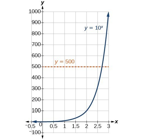
Figure 2

Estimating from a graph, however, is imprecise. To find an algebraic solution, we must introduce a new function. Observe that the graph above passes the horizontal line test. The exponential function [latex]y={b}^{x}[/latex] is one-to-one, so its inverse, [latex]x={b}^{y}[/latex] is also a function. As is the case with all inverse functions, we simply interchange x and y and solve for y to find the inverse function. To represent y as a function of x, we use a logarithmic function of the form [latex]y={\mathrm{log}}_{b}\left(x\right)[/latex]. The base b logarithm of a number is the exponent by which we must raise b to get that number.

We read a logarithmic expression as, “The logarithm with base b of x is equal to y,” or, simplified, “log base b of x is y.” We can also say, “b raised to the power of y is x,” because logs are exponents. For example, the base 2 logarithm of 32 is 5, because 5 is the exponent we must apply to 2 to get 32. Since [latex]{2}^{5}=32[/latex], we can write [latex]{\mathrm{log}}_{2}32=5[/latex]. We read this as “log base 2 of 32 is 5.”

We can express the relationship between logarithmic form and its corresponding exponential form as follows:

Note that the base b is always positive.

Because logarithm is a function, it is most correctly written as [latex]{\mathrm{log}}_{b}\left(x\right)[/latex], using parentheses to denote function evaluation, just as we would with [latex]f\left(x\right)[/latex]. However, when the input is a single variable or number, it is common to see the parentheses dropped and the expression written without parentheses, as [latex]{\mathrm{log}}_{b}x[/latex]. Note that many calculators require parentheses around the x.

We can illustrate the notation of logarithms as follows:

Notice that, comparing the logarithm function and the exponential function, the input and the output are switched. This means [latex]y={\mathrm{log}}_{b}\left(x\right)[/latex] and [latex]y={b}^{x}[/latex] are inverse functions.

 Convert from exponential to logarithmic form

Knowing the squares, cubes, and roots of numbers allows us to evaluate many logarithms mentally. For example, consider [latex]{\mathrm{log}}_{2}8[/latex]. We ask, “To what exponent must 2 be raised in order to get 8?” Because we already know [latex]{2}^{3}=8[/latex], it follows that [latex]{\mathrm{log}}_{2}8=3[/latex].

Now consider solving [latex]{\mathrm{log}}_{7}49[/latex] and [latex]{\mathrm{log}}_{3}27[/latex] mentally.

• We ask, “To what exponent must 7 be raised in order to get 49?” We know [latex]{7}^{2}=49[/latex]. Therefore, [latex]{\mathrm{log}}_{7}49=2[/latex]
• We ask, “To what exponent must 3 be raised in order to get 27?” We know [latex]{3}^{3}=27[/latex]. Therefore, [latex]{\mathrm{log}}_{3}27=3[/latex]

Even some seemingly more complicated logarithms can be evaluated without a calculator. For example, let’s evaluate [latex]{\mathrm{log}}_{\frac{2}{3}}\frac{4}{9}[/latex] mentally.

• We ask, “To what exponent must [latex]\frac{2}{3}[/latex] be raised in order to get [latex]\frac{4}{9}[/latex]? ” We know [latex]{2}^{2}=4[/latex] and [latex]{3}^{2}=9[/latex], so [latex]{\left(\frac{2}{3}\right)}^{2}=\frac{4}{9}[/latex]. Therefore, [latex]{\mathrm{log}}_{\frac{2}{3}}\left(\frac{4}{9}\right)=2[/latex].

 Use common logarithms

The most frequently used base for logarithms is e. Base e logarithms are important in calculus and some scientific applications; they are called natural logarithms. The base e logarithm, [latex]{\mathrm{log}}_{e}\left(x\right)[/latex], has its own notation, [latex]\mathrm{ln}\left(x\right)[/latex].

Most values of [latex]\mathrm{ln}\left(x\right)[/latex] can be found only using a calculator. The major exception is that, because the logarithm of 1 is always 0 in any base, [latex]\mathrm{ln}1=0[/latex]. For other natural logarithms, we can use the [latex]\mathrm{ln}[/latex] key that can be found on most scientific calculators. We can also find the natural logarithm of any power of e using the inverse property of logarithms.

In Graphs of Exponential Functions, we saw how creating a graphical representation of an exponential model gives us another layer of insight for predicting future events. How do logarithmic graphs give us insight into situations? Because every logarithmic function is the inverse function of an exponential function, we can think of every output on a logarithmic graph as the input for the corresponding inverse exponential equation. In other words, logarithms give the cause for an effect.

To illustrate, suppose we invest $2500 in an account that offers an annual interest rate of 5%, compounded continuously. We already know that the balance in our account for any year t can be found with the equation [latex]A=2500{e}^{0.05t}[/latex].

But what if we wanted to know the year for any balance? We would need to create a corresponding new function by interchanging the input and the output; thus we would need to create a logarithmic model for this situation. By graphing the model, we can see the output (year) for any input (account balance). For instance, what if we wanted to know how many years it would take for our initial investment to double? Figure 1 shows this point on the logarithmic graph.

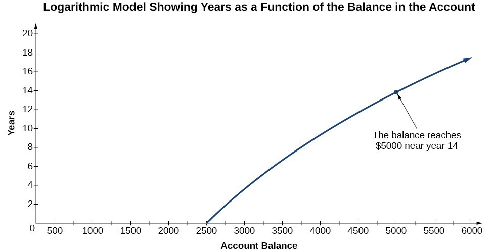
Figure 1

In this section we will discuss the values for which a logarithmic function is defined, and then turn our attention to graphing the family of logarithmic functions.

Identify the domain of a logarithmic function

Before working with graphs, we will take a look at the domain (the set of input values) for which the logarithmic function is defined.

Recall that the exponential function is defined as [latex]y={b}^{x}[/latex] for any real number x and constant [latex]b>0[/latex], [latex]b\ne 1[/latex], where

• The domain of y is [latex]\left(-\infty ,\infty \right)[/latex].
• The range of y is [latex]\left(0,\infty \right)[/latex].

In the last section we learned that the logarithmic function [latex]y={\mathrm{log}}_{b}\left(x\right)[/latex] is the inverse of the exponential function [latex]y={b}^{x}[/latex]. So, as inverse functions:

• The domain of [latex]y={\mathrm{log}}_{b}\left(x\right)[/latex] is the range of [latex]y={b}^{x}[/latex]:[latex]\left(0,\infty \right)[/latex].
• The range of [latex]y={\mathrm{log}}_{b}\left(x\right)[/latex] is the domain of [latex]y={b}^{x}[/latex]: [latex]\left(-\infty ,\infty \right)[/latex].

Transformations of the parent function [latex]y={\mathrm{log}}_{b}\left(x\right)[/latex] behave similarly to those of other functions. Just as with other parent functions, we can apply the four types of transformations—shifts, stretches, compressions, and reflections—to the parent function without loss of shape.

In Graphs of Exponential Functions we saw that certain transformations can change the range of [latex]y={b}^{x}[/latex]. Similarly, applying transformations to the parent function [latex]y={\mathrm{log}}_{b}\left(x\right)[/latex] can change the domain. When finding the domain of a logarithmic function, therefore, it is important to remember that the domain consists only of positive real numbers. That is, the argument of the logarithmic function must be greater than zero.

For example, consider [latex]f\left(x\right)={\mathrm{log}}_{4}\left(2x - 3\right)[/latex]. This function is defined for any values of x such that the argument, in this case [latex]2x - 3[/latex], is greater than zero. To find the domain, we set up an inequality and solve for x:

In interval notation, the domain of [latex]f\left(x\right)={\mathrm{log}}_{4}\left(2x - 3\right)[/latex] is [latex]\left(1.5,\infty \right)[/latex].

 Graph logarithmic functions

Now that we have a feel for the set of values for which a logarithmic function is defined, we move on to graphing logarithmic functions. The family of logarithmic functions includes the parent function [latex]y={\mathrm{log}}_{b}\left(x\right)[/latex] along with all its transformations: shifts, stretches, compressions, and reflections.

We begin with the parent function [latex]y={\mathrm{log}}_{b}\left(x\right)[/latex]. Because every logarithmic function of this form is the inverse of an exponential function with the form [latex]y={b}^{x}[/latex], their graphs will be reflections of each other across the line [latex]y=x[/latex]. To illustrate this, we can observe the relationship between the input and output values of [latex]y={2}^{x}[/latex] and its equivalent [latex]x={\mathrm{log}}_{2}\left(y\right)[/latex] in the table below.

Using the inputs and outputs from the table above, we can build another table to observe the relationship between points on the graphs of the inverse functions [latex]f\left(x\right)={2}^{x}[/latex] and [latex]g\left(x\right)={\mathrm{log}}_{2}\left(x\right)[/latex].

As we’d expect, the x– and y-coordinates are reversed for the inverse functions. The figure below shows the graph of f and g.

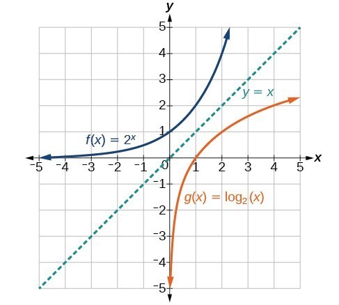
Figure 2. Notice that the graphs of [latex]f\left(x\right)={2}^{x}[/latex] and [latex]g\left(x\right)={\mathrm{log}}_{2}\left(x\right)[/latex] are reflections about the line y = x.

Observe the following from the graph:

• [latex]f\left(x\right)={2}^{x}[/latex] has a y-intercept at [latex]\left(0,1\right)[/latex] and [latex]g\left(x\right)={\mathrm{log}}_{2}\left(x\right)[/latex] has an x-intercept at [latex]\left(1,0\right)[/latex].
• The domain of [latex]f\left(x\right)={2}^{x}[/latex], [latex]\left(-\infty ,\infty \right)[/latex], is the same as the range of [latex]g\left(x\right)={\mathrm{log}}_{2}\left(x\right)[/latex].
• The range of [latex]f\left(x\right)={2}^{x}[/latex], [latex]\left(0,\infty \right)[/latex], is the same as the domain of [latex]g\left(x\right)={\mathrm{log}}_{2}\left(x\right)[/latex].

A General Note: Characteristics of the Graph of the Parent Function, f(x) = log_b(x)

For any real number x and constant b > 0, [latex]b\ne 1[/latex], we can see the following characteristics in the graph of [latex]f\left(x\right)={\mathrm{log}}_{b}\left(x\right)[/latex]:

• one-to-one function
• vertical asymptote: x = 0
• domain: [latex]\left(0,\infty \right)[/latex]
• range: [latex]\left(-\infty ,\infty \right)[/latex]
• x-intercept: [latex]\left(1,0\right)[/latex] and key point [latex]\left(b,1\right)[/latex]
• y-intercept: none
• increasing if [latex]b>1[/latex]
• decreasing if 0 < b < 1

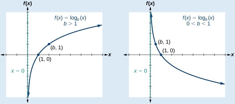
Figure 3 shows how changing the base b in [latex]f\left(x\right)={\mathrm{log}}_{b}\left(x\right)[/latex] can affect the graphs. Observe that the graphs compress vertically as the value of the base increases. (Note: recall that the function [latex]\mathrm{ln}\left(x\right)[/latex] has base [latex]e\approx \text{2}.\text{718.)}[/latex]

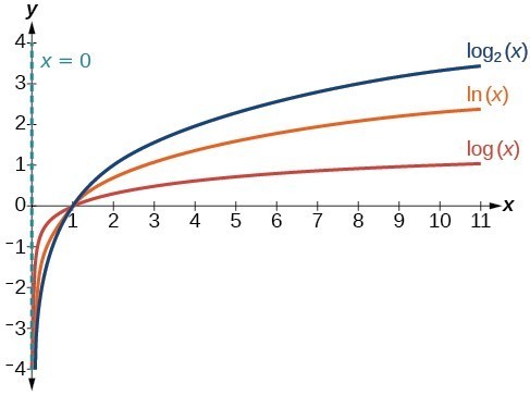
Figure 4. The graphs of three logarithmic functions with different bases, all greater than 1.

Example 3: Graphing a Logarithmic Function with the Form [latex]f\left(x\right)={\mathrm{log}}_{b}\left(x\right)[/latex].

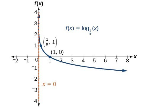
Graph [latex]f\left(x\right)={\mathrm{log}}_{5}\left(x\right)[/latex]. State the domain, range, and asymptote.

Show Solution

Before graphing, identify the behavior and key points for the graph.

• Since b = 5 is greater than one, we know the function is increasing. The left tail of the graph will approach the vertical asymptote x = 0, and the right tail will increase slowly without bound.
• The x-intercept is [latex]\left(1,0\right)[/latex].
• The key point [latex]\left(5,1\right)[/latex] is on the graph.
• We draw and label the asymptote, plot and label the points, and draw a smooth curve through the points.

Figure 5. The domain is [latex]\left(0,\infty \right)[/latex], the range is [latex]\left(-\infty ,\infty \right)[/latex], and the vertical asymptote is x = 0.

 Graphing Transformations of Logarithmic Functions

As we mentioned in the beginning of the section, transformations of logarithmic graphs behave similarly to those of other parent functions. We can shift, stretch, compress, and reflect the parent function [latex]y={\mathrm{log}}_{b}\left(x\right)[/latex] without loss of shape.

Graphing a Horizontal Shift of [latex]f\left(x\right)={\mathrm{log}}_{b}\left(x\right)[/latex]

When a constant c is added to the input of the parent function [latex]f\left(x\right)=\text{log}_{b}\left(x\right)[/latex], the result is a horizontal shift c units in the opposite direction of the sign on c. To visualize horizontal shifts, we can observe the general graph of the parent function [latex]f\left(x\right)={\mathrm{log}}_{b}\left(x\right)[/latex] and for c > 0 alongside the shift left, [latex]g\left(x\right)={\mathrm{log}}_{b}\left(x+c\right)[/latex], and the shift right, [latex]h\left(x\right)={\mathrm{log}}_{b}\left(x-c\right)[/latex].

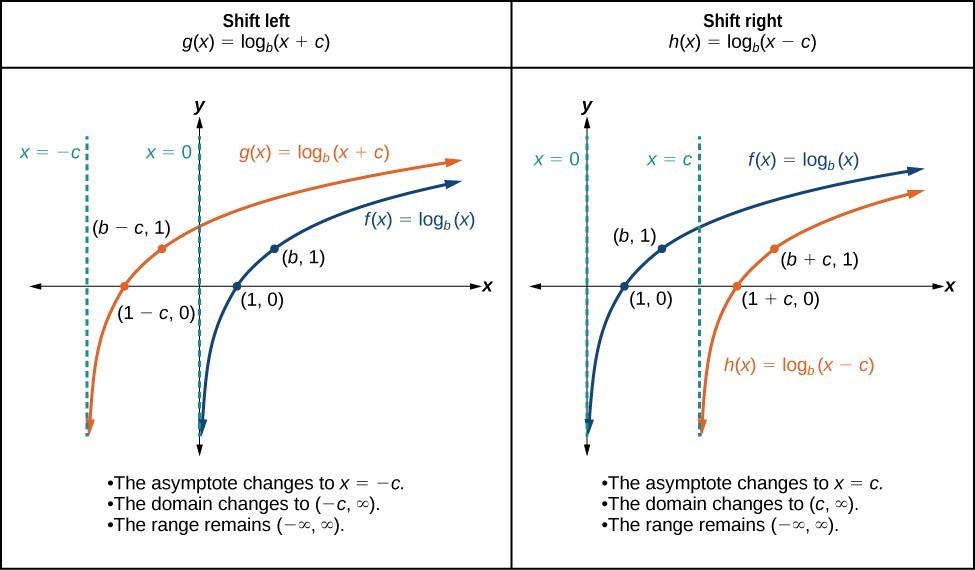
Figure 6

A General Note: Horizontal Shifts of the Parent Function [latex]y=\text{log}_{b}\left(x\right)[/latex]

For any constant c, the function [latex]f\left(x\right)={\mathrm{log}}_{b}\left(x+c\right)[/latex]

• shifts the parent function [latex]y={\mathrm{log}}_{b}\left(x\right)[/latex] left c units if c > 0.
• shifts the parent function [latex]y={\mathrm{log}}_{b}\left(x\right)[/latex] right c units if c < 0.
• has the vertical asymptote x = –c.
• has domain [latex]\left(-c,\infty \right)[/latex].
• has range [latex]\left(-\infty ,\infty \right)[/latex].

How To: Given a logarithmic function with the form [latex]f\left(x\right)={\mathrm{log}}_{b}\left(x+c\right)[/latex], graph the translation.

1. Identify the horizontal shift:
   1. If c > 0, shift the graph of [latex]f\left(x\right)={\mathrm{log}}_{b}\left(x\right)[/latex] left c units.
   2. If c < 0, shift the graph of [latex]f\left(x\right)={\mathrm{log}}_{b}\left(x\right)[/latex] right c units.
2. Draw the vertical asymptote x = –c.
3. Identify three key points from the parent function. Find new coordinates for the shifted functions by subtracting c from the x coordinate.
4. Label the three points.
5. The Domain is [latex]\left(-c,\infty \right)[/latex], the range is [latex]\left(-\infty ,\infty \right)[/latex], and the vertical asymptote is x = –c.

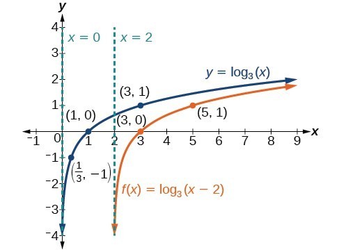
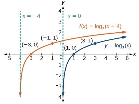
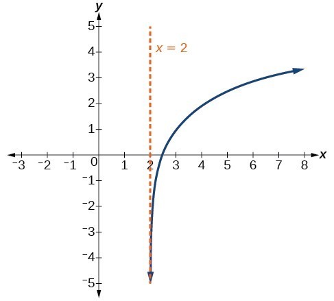
Example 4: Graphing a Horizontal Shift of the Parent Function [latex]y=\text{log}_{b}\left(x\right)[/latex]

Sketch the horizontal shift [latex]f\left(x\right)={\mathrm{log}}_{3}\left(x - 2\right)[/latex] alongside its parent function. Include the key points and asymptotes on the graph. State the domain, range, and asymptote.

Show Solution

Since the function is [latex]f\left(x\right)={\mathrm{log}}_{3}\left(x - 2\right)[/latex], we notice [latex]x+\left(-2\right)=x - 2[/latex].

Thus c = –2, so c < 0. This means we will shift the function [latex]f\left(x\right)={\mathrm{log}}_{3}\left(x\right)[/latex] right 2 units.

The vertical asymptote is [latex]x=-\left(-2\right)[/latex] or x = 2.

Consider the three key points from the parent function, [latex]\left(\frac{1}{3},-1\right)[/latex], [latex]\left(1,0\right)[/latex], and [latex]\left(3,1\right)[/latex].

The new coordinates are found by adding 2 to the x coordinates.

Label the points [latex]\left(\frac{7}{3},-1\right)[/latex], [latex]\left(3,0\right)[/latex], and [latex]\left(5,1\right)[/latex].

The domain is [latex]\left(2,\infty \right)[/latex], the range is [latex]\left(-\infty ,\infty \right)[/latex], and the vertical asymptote is x = 2.

Figure 7

 

Try It

Sketch a graph of [latex]f\left(x\right)={\mathrm{log}}_{3}\left(x+4\right)[/latex] alongside its parent function. Include the key points and asymptotes on the graph. State the domain, range, and asymptote.

Show Solution

The domain is [latex]\left(-4,\infty \right)[/latex], the range [latex]\left(-\infty ,\infty \right)[/latex], and the asymptote x = –4.

Try It

Graphing a Vertical Shift of [latex]y=\text{log}_{b}\left(x\right)[/latex]

When a constant d is added to the parent function [latex]f\left(x\right)={\mathrm{log}}_{b}\left(x\right)[/latex], the result is a vertical shift d units in the direction of the sign on d. To visualize vertical shifts, we can observe the general graph of the parent function [latex]f\left(x\right)={\mathrm{log}}_{b}\left(x\right)[/latex] alongside the shift up, [latex]g\left(x\right)={\mathrm{log}}_{b}\left(x\right)+d[/latex] and the shift down, [latex]h\left(x\right)={\mathrm{log}}_{b}\left(x\right)-d[/latex].

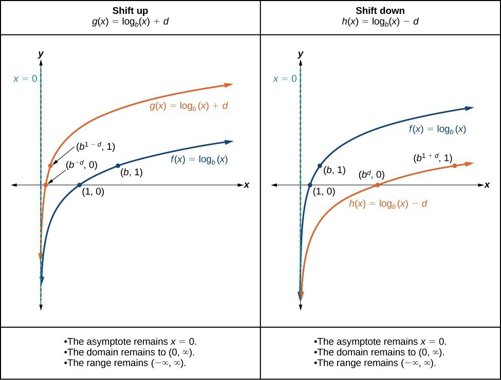
Figure 8

A General Note: Vertical Shifts of the Parent Function [latex]y=\text{log}_{b}\left(x\right)[/latex]

For any constant d, the function [latex]f\left(x\right)={\mathrm{log}}_{b}\left(x\right)+d[/latex]

• shifts the parent function [latex]y={\mathrm{log}}_{b}\left(x\right)[/latex] up d units if d > 0.
• shifts the parent function [latex]y={\mathrm{log}}_{b}\left(x\right)[/latex] down d units if d < 0.
• has the vertical asymptote x = 0.
• has domain [latex]\left(0,\infty \right)[/latex].
• has range [latex]\left(-\infty ,\infty \right)[/latex].

How To: Given a logarithmic function with the form [latex]f\left(x\right)={\mathrm{log}}_{b}\left(x\right)+d[/latex], graph the translation.

1. Identify the vertical shift:
   1. If d > 0, shift the graph of [latex]f\left(x\right)={\mathrm{log}}_{b}\left(x\right)[/latex] up d units.
   2. If d < 0, shift the graph of [latex]f\left(x\right)={\mathrm{log}}_{b}\left(x\right)[/latex] down d units.
2. Draw the vertical asymptote x = 0.
3. Identify three key points from the parent function. Find new coordinates for the shifted functions by adding d to the y coordinate.
4. Label the three points.
5. The domain is [latex]\left(0,\infty \right)[/latex], the range is [latex]\left(-\infty ,\infty \right)[/latex], and the vertical asymptote is x = 0.

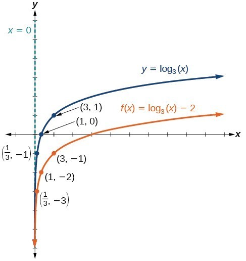
Example 5: Graphing a Vertical Shift of the Parent Function [latex]y=\text{log}_{b}\left(x\right)[/latex]

Sketch a graph of [latex]f\left(x\right)={\mathrm{log}}_{3}\left(x\right)-2[/latex] alongside its parent function. Include the key points and asymptote on the graph. State the domain, range, and asymptote.

Show Solution

Since the function is [latex]f\left(x\right)={\mathrm{log}}_{3}\left(x\right)-2[/latex], we will notice d = –2. Thus d < 0.

This means we will shift the function [latex]f\left(x\right)={\mathrm{log}}_{3}\left(x\right)[/latex] down 2 units.

The vertical asymptote is x = 0.

Consider the three key points from the parent function, [latex]\left(\frac{1}{3},-1\right)[/latex], [latex]\left(1,0\right)[/latex], and [latex]\left(3,1\right)[/latex].

The new coordinates are found by subtracting 2 from the y coordinates.

Label the points [latex]\left(\frac{1}{3},-3\right)[/latex], [latex]\left(1,-2\right)[/latex], and [latex]\left(3,-1\right)[/latex].

The domain is [latex]\left(0,\infty \right)[/latex], the range is [latex]\left(-\infty ,\infty \right)[/latex], and the vertical asymptote is x = 0.

Figure 9. The domain is [latex]\left(0,\infty \right)[/latex], the range is [latex]\left(-\infty ,\infty \right)[/latex], and the vertical asymptote is x = 0.

Try It

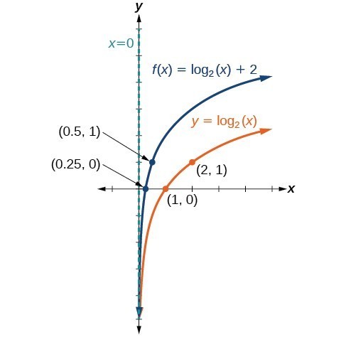
Sketch a graph of [latex]f\left(x\right)={\mathrm{log}}_{2}\left(x\right)+2[/latex] alongside its parent function. Include the key points and asymptote on the graph. State the domain, range, and asymptote.

Show Solution

The domain is [latex]\left(0,\infty \right)[/latex], the range is [latex]\left(-\infty ,\infty \right)[/latex], and the vertical asymptote is x = 0.

Try It

Graphing Stretches and Compressions of [latex]y=\text{log}_{b}\left(x\right)[/latex]

When the parent function [latex]f\left(x\right)={\mathrm{log}}_{b}\left(x\right)[/latex] is multiplied by a constant a > 0, the result is a vertical stretch or compression of the original graph. To visualize stretches and compressions, we set a > 1 and observe the general graph of the parent function [latex]f\left(x\right)={\mathrm{log}}_{b}\left(x\right)[/latex] alongside the vertical stretch, [latex]g\left(x\right)=a{\mathrm{log}}_{b}\left(x\right)[/latex] and the vertical compression, [latex]h\left(x\right)=\frac{1}{a}{\mathrm{log}}_{b}\left(x\right)[/latex].

A General Note: Vertical Stretches and Compressions of the Parent Function [latex]y=\text{log}_{b}\left(x\right)[/latex]

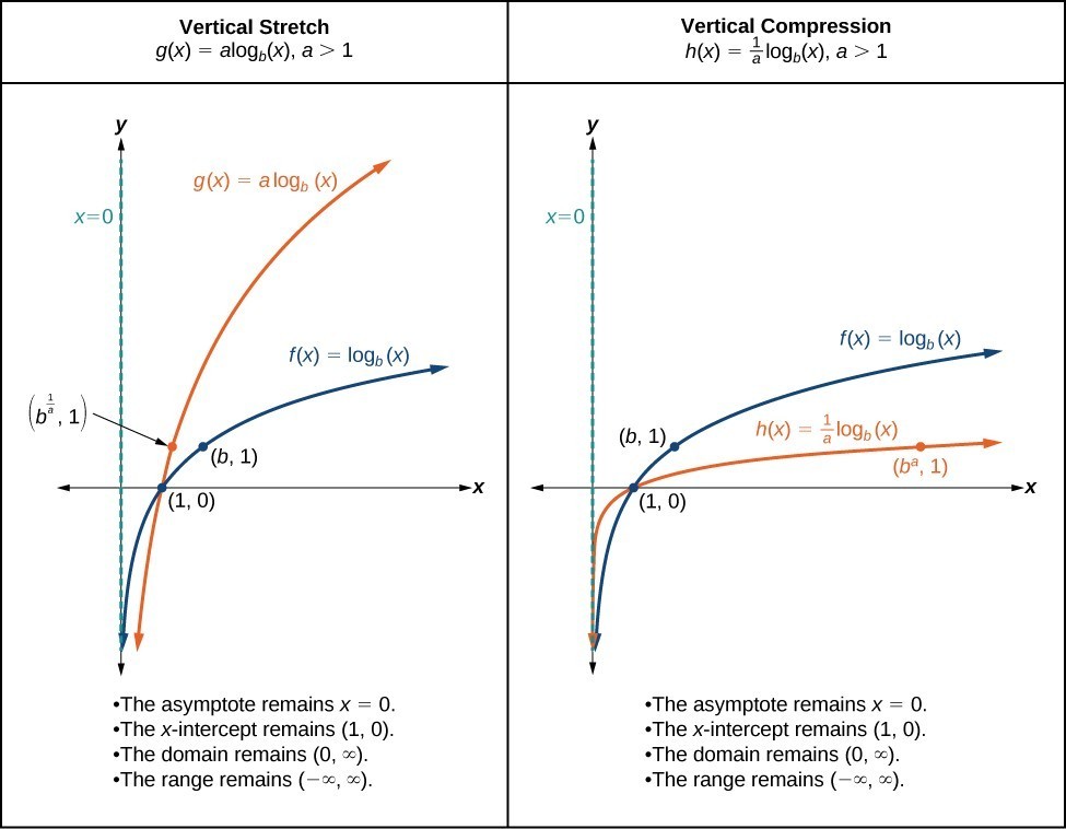
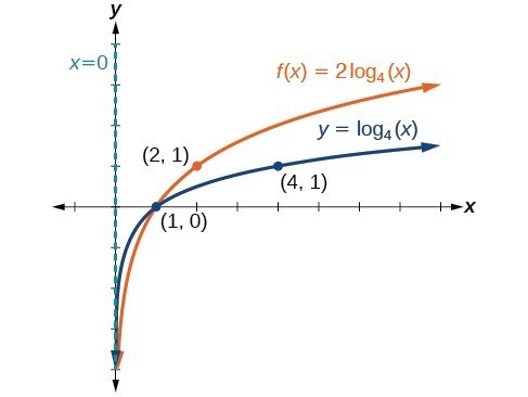
For any constant a > 1, the function [latex]f\left(x\right)=a{\mathrm{log}}_{b}\left(x\right)[/latex]

• stretches the parent function [latex]y={\mathrm{log}}_{b}\left(x\right)[/latex] vertically by a factor of a if a > 1.
• compresses the parent function [latex]y={\mathrm{log}}_{b}\left(x\right)[/latex] vertically by a factor of a if 0 < a < 1.
• has the vertical asymptote x = 0.
• has the x-intercept [latex]\left(1,0\right)[/latex].
• has domain [latex]\left(0,\infty \right)[/latex].
• has range [latex]\left(-\infty ,\infty \right)[/latex].

How To: Given a logarithmic function with the form [latex]f\left(x\right)=a{\mathrm{log}}_{b}\left(x\right)[/latex], [latex]a>0[/latex], graph the translation.

1. Identify the vertical stretch or compressions:
   1. If [latex]|a|>1[/latex], the graph of [latex]f\left(x\right)={\mathrm{log}}_{b}\left(x\right)[/latex] is stretched by a factor of a units.
   2. If [latex]|a|<1[/latex], the graph of [latex]f\left(x\right)={\mathrm{log}}_{b}\left(x\right)[/latex] is compressed by a factor of a units.
2. Draw the vertical asymptote x = 0.
3. Identify three key points from the parent function. Find new coordinates for the shifted functions by multiplying the y coordinates by a.
4. Label the three points.
5. The domain is [latex]\left(0,\infty \right)[/latex], the range is [latex]\left(-\infty ,\infty \right)[/latex], and the vertical asymptote is x = 0.

Example 6: Graphing a Stretch or Compression of the Parent Function [latex]y=\text{log}_{b}\left(x\right)[/latex]

Sketch a graph of [latex]f\left(x\right)=2{\mathrm{log}}_{4}\left(x\right)[/latex] alongside its parent function. Include the key points and asymptote on the graph. State the domain, range, and asymptote.

Show Solution

Since the function is [latex]f\left(x\right)=2{\mathrm{log}}_{4}\left(x\right)[/latex], we will notice a = 2.

This means we will stretch the function [latex]f\left(x\right)={\mathrm{log}}_{4}\left(x\right)[/latex] by a factor of 2.

The vertical asymptote is x = 0.

Consider the three key points from the parent function, [latex]\left(\frac{1}{4},-1\right)[/latex], [latex]\left(1,0\right)[/latex], and [latex]\left(4,1\right)[/latex].

The new coordinates are found by multiplying the y coordinates by 2.

Label the points [latex]\left(\frac{1}{4},-2\right)[/latex], [latex]\left(1,0\right)[/latex], and [latex]\left(4,\text{2}\right)[/latex].

The domain is [latex]\left(0,\infty \right)[/latex], the range is [latex]\left(-\infty ,\infty \right)[/latex], and the vertical asymptote is x = 0.

Figure 11. The domain is [latex]\left(0,\infty \right)[/latex], the range is [latex]\left(-\infty ,\infty \right)[/latex], and the vertical asymptote is x = 0.

Try It

Sketch a graph of [latex]f\left(x\right)=\frac{1}{2}{\mathrm{log}}_{4}\left(x\right)[/latex] alongside its parent function. Include the key points and asymptote on the graph. State the domain, range, and asymptote.

Show Solution

The domain is [latex]\left(0,\infty \right)[/latex], the range is [latex]\left(-\infty ,\infty \right)[/latex], and the vertical asymptote is x = 0.

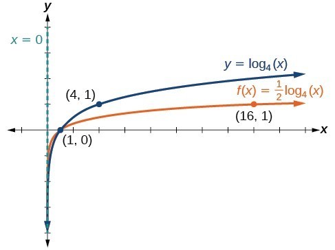
Example 7: Combining a Shift and a Stretch

Sketch a graph of [latex]f\left(x\right)=5\mathrm{log}\left(x+2\right)[/latex]. State the domain, range, and asymptote.

Show Solution

Remember: what happens inside parentheses happens first. First, we move the graph left 2 units, then stretch the function vertically by a factor of 5. The vertical asymptote will be shifted to x = –2. The x-intercept will be [latex]\left(-1,0\right)[/latex]. The domain will be [latex]\left(-2,\infty \right)[/latex]. Two points will help give the shape of the graph: [latex]\left(-1,0\right)[/latex] and [latex]\left(8,5\right)[/latex]. We chose x = 8 as the x-coordinate of one point to graph because when x = 8, x + 2 = 10, the base of the common logarithm.

Figure 12. The domain is [latex]\left(-2,\infty \right)[/latex], the range is [latex]\left(-\infty ,\infty \right)[/latex], and the vertical asymptote is x = –2.

Try It

Sketch a graph of the function [latex]f\left(x\right)=3\mathrm{log}\left(x - 2\right)+1[/latex]. State the domain, range, and asymptote.

Show Solution

The domain is [latex]\left(2,\infty \right)[/latex], the range is [latex]\left(-\infty ,\infty \right)[/latex], and the vertical asymptote is x = 2.

Try It

Graphing Reflections of [latex]f\left(x\right)={\mathrm{log}}_{b}\left(x\right)[/latex]

When the parent function [latex]f\left(x\right)={\mathrm{log}}_{b}\left(x\right)[/latex] is multiplied by –1, the result is a reflection about the x-axis. When the input is multiplied by –1, the result is a reflection about the y-axis. To visualize reflections, we restrict b > 1, and observe the general graph of the parent function [latex]f\left(x\right)={\mathrm{log}}_{b}\left(x\right)[/latex] alongside the reflection about the x-axis, [latex]g\left(x\right)={\mathrm{-log}}_{b}\left(x\right)[/latex] and the reflection about the y-axis, [latex]h\left(x\right)={\mathrm{log}}_{b}\left(-x\right)[/latex].

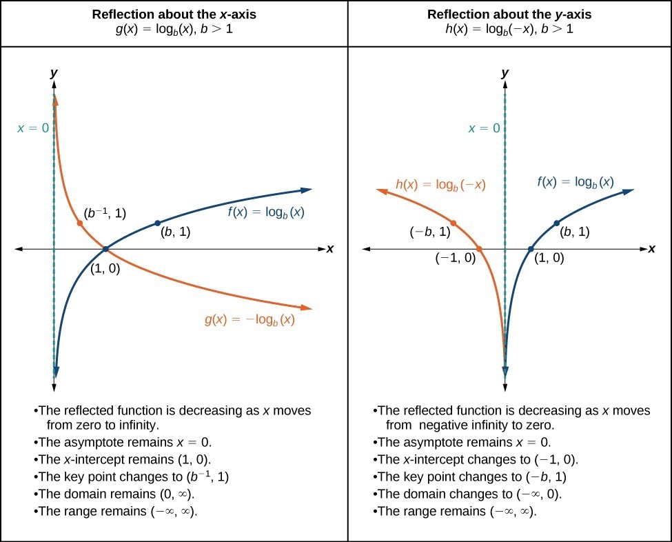
A General Note: Reflections of the Parent Function [latex]y=\text{log}_{b}\left(x\right)[/latex]

The function [latex]f\left(x\right)={\mathrm{-log}}_{b}\left(x\right)[/latex]

• reflects the parent function [latex]y={\mathrm{log}}_{b}\left(x\right)[/latex] about the x-axis.
• has domain, [latex]\left(0,\infty \right)[/latex], range, [latex]\left(-\infty ,\infty \right)[/latex], and vertical asymptote, x = 0, which are unchanged from the parent function.

The function [latex]f\left(x\right)={\mathrm{log}}_{b}\left(-x\right)[/latex]

• reflects the parent function [latex]y={\mathrm{log}}_{b}\left(x\right)[/latex] about the y-axis.
• has domain [latex]\left(-\infty ,0\right)[/latex].
• has range, [latex]\left(-\infty ,\infty \right)[/latex], and vertical asymptote, x = 0, which are unchanged from the parent function.

How To: Given a logarithmic function with the parent function [latex]f\left(x\right)={\mathrm{log}}_{b}\left(x\right)[/latex], graph a translation.

[latex]\text{If }f\left(x\right)=-{\mathrm{log}}_{b}\left(x\right)[/latex]	[latex]\text{If }f\left(x\right)={\mathrm{log}}_{b}\left(-x\right)[/latex]
1. Draw the vertical asymptote, x = 0.	1. Draw the vertical asymptote, x = 0.
2. Plot the x-intercept, [latex]\left(1,0\right)[/latex].	2. Plot the x-intercept, [latex]\left(1,0\right)[/latex].
3. Reflect the graph of the parent function [latex]f\left(x\right)={\mathrm{log}}_{b}\left(x\right)[/latex] about the x-axis.	3. Reflect the graph of the parent function [latex]f\left(x\right)={\mathrm{log}}_{b}\left(x\right)[/latex] about the y-axis.
4. Draw a smooth curve through the points.	4. Draw a smooth curve through the points.
5. State the domain, [latex]\left(0,\infty \right)[/latex], the range, [latex]\left(-\infty ,\infty \right)[/latex], and the vertical asymptote x = 0.	5. State the domain, [latex]\left(-\infty ,0\right)[/latex], the range, [latex]\left(-\infty ,\infty \right)[/latex], and the vertical asymptote x = 0.

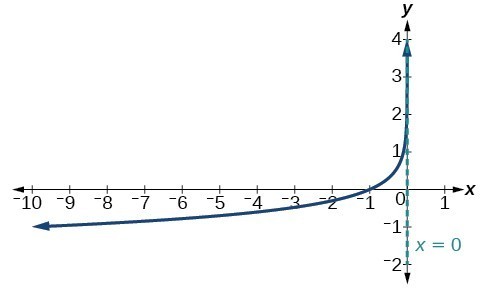
Example 8: Graphing a Reflection of a Logarithmic Function

Sketch a graph of [latex]f\left(x\right)=\mathrm{log}\left(-x\right)[/latex] alongside its parent function. Include the key points and asymptote on the graph. State the domain, range, and asymptote.

Show Solution

Before graphing [latex]f\left(x\right)=\mathrm{log}\left(-x\right)[/latex], identify the behavior and key points for the graph.

• Since b = 10 is greater than one, we know that the parent function is increasing. Since the input value is multiplied by –1, f is a reflection of the parent graph about the y-axis. Thus, [latex]f\left(x\right)=\mathrm{log}\left(-x\right)[/latex] will be decreasing as x moves from negative infinity to zero, and the right tail of the graph will approach the vertical asymptote x = 0.
• The x-intercept is [latex]\left(-1,0\right)[/latex].
• We draw and label the asymptote, plot and label the points, and draw a smooth curve through the points.

Figure 14. The domain is [latex]\left(-\infty ,0\right)[/latex], the range is [latex]\left(-\infty ,\infty \right)[/latex], and the vertical asymptote is x = 0.

Try It

Graph [latex]f\left(x\right)=-\mathrm{log}\left(-x\right)[/latex]. State the domain, range, and asymptote.

Show Solution

The domain is [latex]\left(-\infty ,0\right)[/latex], the range is [latex]\left(-\infty ,\infty \right)[/latex], and the vertical asymptote is x = 0.

How To: Given a logarithmic equation, use a graphing calculator to approximate solutions.

1. Press [Y=]. Enter the given logarithm equation or equations as Y₁= and, if needed, Y₂=.
2. Press [GRAPH] to observe the graphs of the curves and use [WINDOW] to find an appropriate view of the graphs, including their point(s) of intersection.
3. To find the value of x, we compute the point of intersection. Press [2ND] then [CALC]. Select “intersect” and press [ENTER] three times. The point of intersection gives the value of x, for the point(s) of intersection.

Example 9: Approximating the Solution of a Logarithmic Equation

Solve [latex]4\mathrm{ln}\left(x\right)+1=-2\mathrm{ln}\left(x - 1\right)[/latex] graphically. Round to the nearest thousandth.

Show Solution

Press [Y=] and enter [latex]4\mathrm{ln}\left(x\right)+1[/latex] next to Y₁=. Then enter [latex]-2\mathrm{ln}\left(x - 1\right)[/latex] next to Y₂=. For a window, use the values 0 to 5 for x and –10 to 10 for y. Press [GRAPH]. The graphs should intersect somewhere a little to right of x = 1.

For a better approximation, press [2ND] then [CALC]. Select [5: intersect] and press [ENTER] three times. The x-coordinate of the point of intersection is displayed as 1.3385297. (Your answer may be different if you use a different window or use a different value for Guess?) So, to the nearest thousandth, [latex]x\approx 1.339[/latex].

Try It

Solve [latex]5\mathrm{log}\left(x+2\right)=4-\mathrm{log}\left(x\right)[/latex] graphically. Round to the nearest thousandth.

Show Solution

[latex]x\approx 3.049[/latex]

Summarizing Translations of the Logarithmic Function

Now that we have worked with each type of translation for the logarithmic function, we can summarize each in the table below to arrive at the general equation for translating exponential functions.

Translations of the Parent Function [latex]y={\mathrm{log}}_{b}\left(x\right)[/latex]
Translation	Form
Shift Horizontally c units to the left Vertically d units up	[latex]y={\mathrm{log}}_{b}\left(x+c\right)+d[/latex]
Stretch and Compress Stretch if [latex]|a|>1[/latex] Compression if [latex]|a|<1[/latex]	[latex]y=a{\mathrm{log}}_{b}\left(x\right)[/latex]
Reflect about the x-axis	[latex]y=-{\mathrm{log}}_{b}\left(x\right)[/latex]
Reflect about the y-axis	[latex]y={\mathrm{log}}_{b}\left(-x\right)[/latex]
General equation for all translations	[latex]y=a{\mathrm{log}}_{b}\left(x+c\right)+d[/latex]

A General Note: Translations of Logarithmic Functions

All translations of the parent logarithmic function, [latex]y={\mathrm{log}}_{b}\left(x\right)[/latex], have the form

[latex] f\left(x\right)=a{\mathrm{log}}_{b}\left(x+c\right)+d[/latex]

where the parent function, [latex]y={\mathrm{log}}_{b}\left(x\right),b>1[/latex], is

• shifted vertically up d units.
• shifted horizontally to the left c units.
• stretched vertically by a factor of |a| if |a| > 0.
• compressed vertically by a factor of |a| if 0 < |a| < 1.
• reflected about the x-axis when a < 0.

For [latex]f\left(x\right)=\mathrm{log}\left(-x\right)[/latex], the graph of the parent function is reflected about the y-axis.

Example 10: Finding the Vertical Asymptote of a Logarithm Graph

What is the vertical asymptote of [latex]f\left(x\right)=-2{\mathrm{log}}_{3}\left(x+4\right)+5[/latex]?

Show Solution

The vertical asymptote is at x = –4.

Analysis of the Solution

The coefficient, the base, and the upward translation do not affect the asymptote. The shift of the curve 4 units to the left shifts the vertical asymptote to x = –4.

Try It

What is the vertical asymptote of [latex]f\left(x\right)=3+\mathrm{ln}\left(x - 1\right)[/latex]?

Show Solution

x = 1

Example 11: Finding the Equation from a Graph

Find a possible equation for the common logarithmic function graphed in Figure 15.

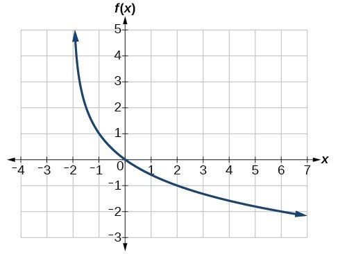
Figure 15

Show Solution

This graph has a vertical asymptote at x = –2 and has been vertically reflected. We do not know yet the vertical shift or the vertical stretch. We know so far that the equation will have form:

[latex]f\left(x\right)=-a\mathrm{log}\left(x+2\right)+k[/latex]

It appears the graph passes through the points [latex]\left(-1,1\right)[/latex] and [latex]\left(2,-1\right)[/latex]. Substituting [latex]\left(-1,1\right)[/latex],

[latex]\begin{align}&1=-a\mathrm{log}\left(-1+2\right)+k && \text{Substitute }\left(-1,1\right). \\ &1=-a\mathrm{log}\left(1\right)+k && \text{Arithmetic}. \\ &1=k && \text{log(1)}=0. \end{align}[/latex]

Next, substituting in [latex]\left(2,-1\right)[/latex],

[latex]\begin{align}&-1=-a\mathrm{log}\left(2+2\right)+1 && \text{Plug in }\left(2,-1\right). \\ &-2=-a\mathrm{log}\left(4\right) && \text{Arithmetic}. \\ &a=\frac{2}{\mathrm{log}\left(4\right)}&& \text{Solve for }a. \end{align}[/latex]

This gives us the equation [latex]f\left(x\right)=-\frac{2}{\mathrm{log}\left(4\right)}\mathrm{log}\left(x+2\right)+1[/latex].

Analysis of the Solution

We can verify this answer by comparing the function values in the table below with the points on the graph in Example 11.

x	−1	0	1	2	3
f(x)	1	0	−0.58496	−1	−1.3219
x	4	5	6	7	8
f(x)	−1.5850	−1.8074	−2	−2.1699	−2.3219

Try It

Give the equation of the natural logarithm graphed in Figure 16.

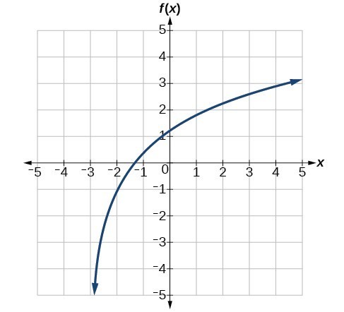
Figure 16

Show Solution

[latex]f\left(x\right)=2\mathrm{ln}\left(x+3\right)-1[/latex]

Q & A

Is it possible to tell the domain and range and describe the end behavior of a function just by looking at the graph?

Yes, if we know the function is a general logarithmic function. For example, look at the graph in Try It 11. The graph approaches x = –3 (or thereabouts) more and more closely, so x = –3 is, or is very close to, the vertical asymptote. It approaches from the right, so the domain is all points to the right, [latex]\left\{x|x>-3\right\}[/latex]. The range, as with all general logarithmic functions, is all real numbers. And we can see the end behavior because the graph goes down as it goes left and up as it goes right. The end behavior is that as [latex]x\to -{3}^{+},f\left(x\right)\to -\infty [/latex] and as [latex]x\to \infty ,f\left(x\right)\to \infty [/latex].

Figure 1. The pH of hydrochloric acid is tested with litmus paper. (credit: David Berardan)

In chemistry, pH is used as a measure of the acidity or alkalinity of a substance. The pH scale runs from 0 to 14. Substances with a pH less than 7 are considered acidic, and substances with a pH greater than 7 are said to be alkaline. Our bodies, for instance, must maintain a pH close to 7.35 in order for enzymes to work properly. To get a feel for what is acidic and what is alkaline, consider the following pH levels of some common substances:

• Battery acid: 0.8
• Stomach acid: 2.7
• Orange juice: 3.3
• Pure water: 7 (at 25° C)
• Human blood: 7.35
• Fresh coconut: 7.8
• Sodium hydroxide (lye): 14

To determine whether a solution is acidic or alkaline, we find its pH, which is a measure of the number of active positive hydrogen ions in the solution. The pH is defined by the following formula, where a is the concentration of hydrogen ion in the solution

The equivalence of [latex]-\mathrm{log}\left(\left[{H}^{+}\right]\right)[/latex] and [latex]\mathrm{log}\left(\frac{1}{\left[{H}^{+}\right]}\right)[/latex] is one of the logarithm properties we will examine in this section.

Use the product rule for logarithms

Recall that the logarithmic and exponential functions “undo” each other. This means that logarithms have similar properties to exponents. Some important properties of logarithms are given here. First, the following properties are easy to prove.

For example, [latex]{\mathrm{log}}_{5}1=0[/latex] since [latex]{5}^{0}=1[/latex]. And [latex]{\mathrm{log}}_{5}5=1[/latex] since [latex]{5}^{1}=5[/latex].

Next, we have the inverse property.

For example, to evaluate [latex]\mathrm{log}\left(100\right)[/latex], we can rewrite the logarithm as [latex]{\mathrm{log}}_{10}\left({10}^{2}\right)[/latex], and then apply the inverse property [latex]{\mathrm{log}}_{b}\left({b}^{x}\right)=x[/latex] to get [latex]{\mathrm{log}}_{10}\left({10}^{2}\right)=2[/latex].

To evaluate [latex]{e}^{\mathrm{ln}\left(7\right)}[/latex], we can rewrite the logarithm as [latex]{e}^{{\mathrm{log}}_{e}7}[/latex], and then apply the inverse property [latex]{b}^{{\mathrm{log}}_{b}x}=x[/latex] to get [latex]{e}^{{\mathrm{log}}_{e}7}=7[/latex].

Finally, we have the one-to-one property.

We can use the one-to-one property to solve the equation [latex]{\mathrm{log}}_{3}\left(3x\right)={\mathrm{log}}_{3}\left(2x+5\right)[/latex] for x. Since the bases are the same, we can apply the one-to-one property by setting the arguments equal and solving for x:

But what about the equation [latex]{\mathrm{log}}_{3}\left(3x\right)+{\mathrm{log}}_{3}\left(2x+5\right)=2[/latex]? The one-to-one property does not help us in this instance. Before we can solve an equation like this, we need a method for combining terms on the left side of the equation.

Recall that we use the product rule of exponents to combine the product of exponents by adding: [latex]{x}^{a}{x}^{b}={x}^{a+b}[/latex]. We have a similar property for logarithms, called the product rule for logarithms, which says that the logarithm of a product is equal to a sum of logarithms. Because logs are exponents, and we multiply like bases, we can add the exponents. We will use the inverse property to derive the product rule below.

Given any real number x and positive real numbers M, N, and b, where [latex]b\ne 1[/latex], we will show

Let [latex]m={\mathrm{log}}_{b}M[/latex] and [latex]n={\mathrm{log}}_{b}N[/latex]. In exponential form, these equations are [latex]{b}^{m}=M[/latex] and [latex]{b}^{n}=N[/latex]. It follows that

Note that repeated applications of the product rule for logarithms allow us to simplify the logarithm of the product of any number of factors. For example, consider [latex]{\mathrm{log}}_{b}\left(wxyz\right)[/latex]. Using the product rule for logarithms, we can rewrite this logarithm of a product as the sum of logarithms of its factors:

Use the quotient and power rules for logarithms

We can use the rules of logarithms we just learned to condense sums, differences, and products with the same base as a single logarithm. It is important to remember that the logarithms must have the same base to be combined. We will learn later how to change the base of any logarithm before condensing.

 Use the change-of-base formula for logarithms

Key Equations