Learning Outcomes
- Build an exponential model from data.
- Build a logarithmic model from data.
- Build a logistic model from data.
In previous sections of this chapter, we were either given a function explicitly to graph or evaluate, or we were given a set of points that were guaranteed to lie on the curve. Then we used algebra to find the equation that fit the points exactly. In this section, we use a modeling technique called regression analysis to find a curve that models data collected from real-world observations. With regression analysis, we don’t expect all the points to lie perfectly on the curve. The idea is to find a model that best fits the data. Then we use the model to make predictions about future events.
Do not be confused by the word model. In mathematics, we often use the terms function, equation, and model interchangeably, even though they each have their own formal definition. The term model is typically used to indicate that the equation or function approximates a real-world situation.
We will concentrate on three types of regression models in this section: exponential, logarithmic, and logistic. Having already worked with each of these functions gives us an advantage. Knowing their formal definitions, the behavior of their graphs, and some of their real-world applications gives us the opportunity to deepen our understanding. As each regression model is presented, key features and definitions of its associated function are included for review. Take a moment to rethink each of these functions, reflect on the work we’ve done so far, and then explore the ways regression is used to model real-world phenomena.
Build an exponential model from data
As we’ve learned, there are a multitude of situations that can be modeled by exponential functions, such as investment growth, radioactive decay, atmospheric pressure changes, and temperatures of a cooling object. What do these phenomena have in common? For one thing, all the models either increase or decrease as time moves forward. But that’s not the whole story. It’s the way data increase or decrease that helps us determine whether it is best modeled by an exponential equation. Knowing the behavior of exponential functions in general allows us to recognize when to use exponential regression, so let’s review exponential growth and decay.
Recall that exponential functions have the form [latex]y=a{b}^{x}[/latex] or [latex]y={A}_{0}{e}^{kx}[/latex]. When performing regression analysis, we use the form most commonly used on graphing utilities, [latex]y=a{b}^{x}[/latex]. Take a moment to reflect on the characteristics we’ve already learned about the exponential function [latex]y=a{b}^{x}[/latex] (assume a > 0):
- b must be greater than zero and not equal to one.
- The initial value of the model is y = a.
- If b > 1, the function models exponential growth. As x increases, the outputs of the model increase slowly at first, but then increase more and more rapidly, without bound.
- If 0 < b < 1, the function models exponential decay. As x increases, the outputs for the model decrease rapidly at first and then level off to become asymptotic to the x-axis. In other words, the outputs never become equal to or less than zero.
As part of the results, your calculator will display a number known as the correlation coefficient, labeled by the variable r, or [latex]{r}^{2}[/latex]. (You may have to change the calculator’s settings for these to be shown.) The values are an indication of the “goodness of fit” of the regression equation to the data. We more commonly use the value of [latex]{r}^{2}[/latex] instead of r, but the closer either value is to 1, the better the regression equation approximates the data.
A General Note: Exponential Regression
Exponential regression is used to model situations in which growth begins slowly and then accelerates rapidly without bound, or where decay begins rapidly and then slows down to get closer and closer to zero. We use the command “ExpReg” on a graphing utility to fit an exponential function to a set of data points. This returns an equation of the form, [latex]y=a{b}^{x}[/latex]
Note that:
- b must be non-negative.
- when b > 1, we have an exponential growth model.
- when 0 < b < 1, we have an exponential decay model.
How To: Given a set of data, perform exponential regression using a graphing utility.
- Use the STAT then EDIT menu to enter given data.
- Clear any existing data from the lists.
- List the input values in the L1 column.
- List the output values in the L2 column.
- Graph and observe a scatter plot of the data using the STATPLOT feature.
- Use ZOOM [9] to adjust axes to fit the data.
- Verify the data follow an exponential pattern.
- Find the equation that models the data.
- Select “ExpReg” from the STAT then CALC menu.
- Use the values returned for a and b to record the model, [latex]y=a{b}^{x}[/latex].
- Graph the model in the same window as the scatterplot to verify it is a good fit for the data.
Example 1: Using Exponential Regression to Fit a Model to Data
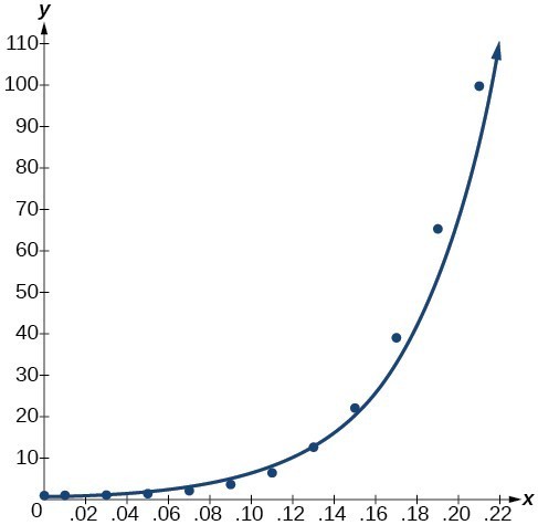
In 2007, a university study was published investigating the crash risk of alcohol impaired driving. Data from 2,871 crashes were used to measure the association of a person’s blood alcohol level (BAC) with the risk of being in an accident. The table below shows results from the study.[1] The relative risk is a measure of how many times more likely a person is to crash. So, for example, a person with a BAC of 0.09 is 3.54 times as likely to crash as a person who has not been drinking alcohol.
| BAC | 0 | 0.01 | 0.03 | 0.05 | 0.07 | 0.09 |
| Relative Risk of Crashing | 1 | 1.03 | 1.06 | 1.38 | 2.09 | 3.54 |
| BAC | 0.11 | 0.13 | 0.15 | 0.17 | 0.19 | 0.21 |
| Relative Risk of Crashing | 6.41 | 12.6 | 22.1 | 39.05 | 65.32 | 99.78 |
- Let x represent the BAC level, and let y represent the corresponding relative risk. Use exponential regression to fit a model to these data.
- After 6 drinks, a person weighing 160 pounds will have a BAC of about 0.16. How many times more likely is a person with this weight to crash if they drive after having a 6-pack of beer? Round to the nearest hundredth.

Try It
The table below shows a recent graduate’s credit card balance each month after graduation.
| Month | 1 | 2 | 3 | 4 | 5 | 6 | 7 | 8 |
| Debt ($) | 620.00 | 761.88 | 899.80 | 1039.93 | 1270.63 | 1589.04 | 1851.31 | 2154.92 |
a. Use exponential regression to fit a model to these data.
b. If spending continues at this rate, what will the graduate’s credit card debt be one year after graduating?
Q & A
Is it reasonable to assume that an exponential regression model will represent a situation indefinitely?
No. Remember that models are formed by real-world data gathered for regression. It is usually reasonable to make estimates within the interval of original observation (interpolation). However, when a model is used to make predictions, it is important to use reasoning skills to determine whether the model makes sense for inputs far beyond the original observation interval (extrapolation).
Build a logarithmic model from data
Just as with exponential functions, there are many real-world applications for logarithmic functions: intensity of sound, pH levels of solutions, yields of chemical reactions, production of goods, and growth of infants. As with exponential models, data modeled by logarithmic functions are either always increasing or always decreasing as time moves forward. Again, it is the way they increase or decrease that helps us determine whether a logarithmic model is best.
Recall that logarithmic functions increase or decrease rapidly at first, but then steadily slow as time moves on. By reflecting on the characteristics we’ve already learned about this function, we can better analyze real world situations that reflect this type of growth or decay. When performing logarithmic regression analysis, we use the form of the logarithmic function most commonly used on graphing utilities, [latex]y=a+b\mathrm{ln}\left(x\right)[/latex]. For this function
- All input values, x, must be greater than zero.
- The point (1, a) is on the graph of the model.
- If b > 0, the model is increasing. Growth increases rapidly at first and then steadily slows over time.
- If b < 0, the model is decreasing. Decay occurs rapidly at first and then steadily slows over time.
A General Note: Logarithmic Regression
Logarithmic regression is used to model situations where growth or decay accelerates rapidly at first and then slows over time. We use the command “LnReg” on a graphing utility to fit a logarithmic function to a set of data points. This returns an equation of the form,
Note that
- all input values, x, must be non-negative.
- when b > 0, the model is increasing.
- when b < 0, the model is decreasing.
How To: Given a set of data, perform logarithmic regression using a graphing utility.
- Use the STAT then EDIT menu to enter given data.
- Clear any existing data from the lists.
- List the input values in the L1 column.
- List the output values in the L2 column.
- Graph and observe a scatter plot of the data using the STATPLOT feature.
- Use ZOOM [9] to adjust axes to fit the data.
- Verify the data follow a logarithmic pattern.
- Find the equation that models the data.
- Select “LnReg” from the STAT then CALC menu.
- Use the values returned for a and b to record the model, [latex]y=a+b\mathrm{ln}\left(x\right)[/latex].
- Graph the model in the same window as the scatterplot to verify it is a good fit for the data.
Example 2: Using Logarithmic Regression to Fit a Model to Data
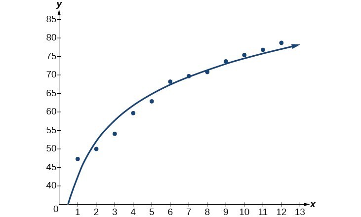
Due to advances in medicine and higher standards of living, life expectancy has been increasing in most developed countries since the beginning of the 20th century.
The table below shows the average life expectancies, in years, of Americans from 1900–2010.[2]
| Year | 1900 | 1910 | 1920 | 1930 | 1940 | 1950 |
| Life Expectancy(Years) | 47.3 | 50.0 | 54.1 | 59.7 | 62.9 | 68.2 |
| Year | 1960 | 1970 | 1980 | 1990 | 2000 | 2010 |
| Life Expectancy(Years) | 69.7 | 70.8 | 73.7 | 75.4 | 76.8 | 78.7 |
- Let x represent time in decades starting with x = 1 for the year 1900, x = 2 for the year 1910, and so on. Let y represent the corresponding life expectancy. Use logarithmic regression to fit a model to these data.
- Use the model to predict the average American life expectancy for the year 2030.

Try It
Sales of a video game released in the year 2000 took off at first, but then steadily slowed as time moved on. The table below shows the number of games sold, in thousands, from the years 2000–2010.
| Year | 2000 | 2001 | 2002 | 2003 | 2004 | 2005 |
| Number Sold (thousands) | 142 | 149 | 154 | 155 | 159 | 161 |
| Year | 2006 | 2007 | 2008 | 2009 | 2010 | — |
| Number Sold (thousands) | 163 | 164 | 164 | 166 | 167 | — |
a. Let x represent time in years starting with x = 1 for the year 2000. Let y represent the number of games sold in thousands. Use logarithmic regression to fit a model to these data.
b. If games continue to sell at this rate, how many games will sell in 2015? Round to the nearest thousand.
Build a logistic model from data
Like exponential and logarithmic growth, logistic growth increases over time. One of the most notable differences with logistic growth models is that, at a certain point, growth steadily slows and the function approaches an upper bound, or limiting value. Because of this, logistic regression is best for modeling phenomena where there are limits in expansion, such as availability of living space or nutrients.
It is worth pointing out that logistic functions actually model resource-limited exponential growth. There are many examples of this type of growth in real-world situations, including population growth and spread of disease, rumors, and even stains in fabric. When performing logistic regression analysis, we use the form most commonly used on graphing utilities:
Recall that:
- [latex]\frac{c}{1+a}[/latex] is the initial value of the model.
- when b > 0, the model increases rapidly at first until it reaches its point of maximum growth rate, [latex]\left(\frac{\mathrm{ln}\left(a\right)}{b},\frac{c}{2}\right)[/latex]. At that point, growth steadily slows and the function becomes asymptotic to the upper bound y = c.
- c is the limiting value, sometimes called the carrying capacity, of the model.
A General Note: Logistic Regression
Logistic regression is used to model situations where growth accelerates rapidly at first and then steadily slows to an upper limit. We use the command “Logistic” on a graphing utility to fit a logistic function to a set of data points. This returns an equation of the form
Note that
- The initial value of the model is [latex]\frac{c}{1+a}[/latex].
- Output values for the model grow closer and closer to y = c as time increases.
How To: Given a set of data, perform logistic regression using a graphing utility.
- Use the STAT then EDIT menu to enter given data.
- Clear any existing data from the lists.
- List the input values in the L1 column.
- List the output values in the L2 column.
- Graph and observe a scatter plot of the data using the STATPLOT feature.
- Use ZOOM [9] to adjust axes to fit the data.
- Verify the data follow a logistic pattern.
- Find the equation that models the data.
- Select “Logistic” from the STAT then CALC menu.
- Use the values returned for a, b, and c to record the model, [latex]y=\frac{c}{1+a{e}^{-bx}}[/latex].
- Graph the model in the same window as the scatterplot to verify it is a good fit for the data.
Example 3: Using Logistic Regression to Fit a Model to Data
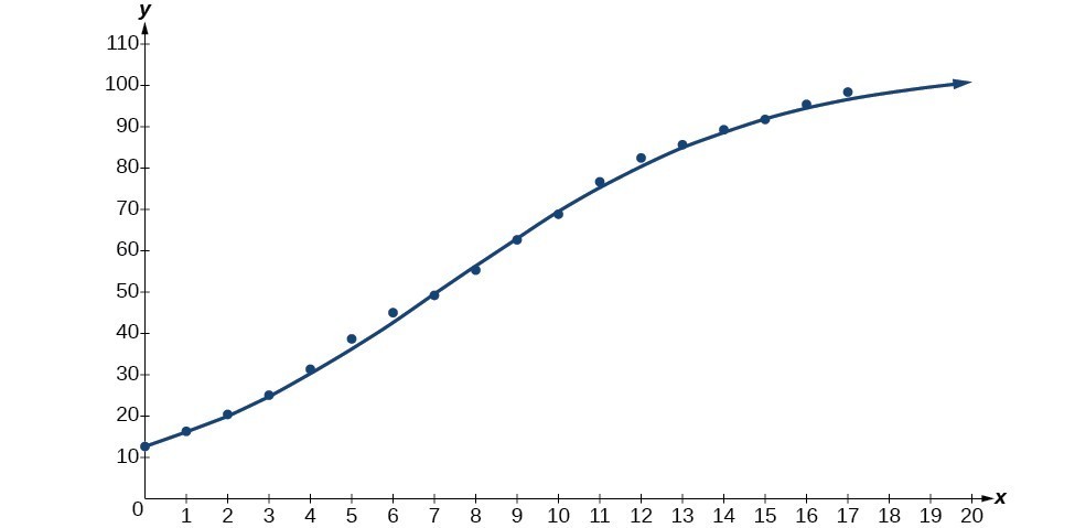
Mobile telephone service has increased rapidly in America since the mid 1990s. Today, almost all residents have cellular service. The table below shows the percentage of Americans with cellular service between the years 1995 and 2012.[3]
| Year | Americans with Cellular Service (%) | Year | Americans with Cellular Service (%) |
|---|---|---|---|
| 1995 | 12.69 | 2004 | 62.852 |
| 1996 | 16.35 | 2005 | 68.63 |
| 1997 | 20.29 | 2006 | 76.64 |
| 1998 | 25.08 | 2007 | 82.47 |
| 1999 | 30.81 | 2008 | 85.68 |
| 2000 | 38.75 | 2009 | 89.14 |
| 2001 | 45.00 | 2010 | 91.86 |
| 2002 | 49.16 | 2011 | 95.28 |
| 2003 | 55.15 | 2012 | 98.17 |
- Let x represent time in years starting with x = 0 for the year 1995. Let y represent the corresponding percentage of residents with cellular service. Use logistic regression to fit a model to these data.
- Use the model to calculate the percentage of Americans with cell service in the year 2013. Round to the nearest tenth of a percent.
- Discuss the value returned for the upper limit, c. What does this tell you about the model? What would the limiting value be if the model were exact?

Try It
The table below shows the population, in thousands, of harbor seals in the Wadden Sea over the years 1997 to 2012.
| Year | Seal Population (Thousands) | Year | Seal Population (Thousands) |
|---|---|---|---|
| 1997 | 3.493 | 2005 | 19.590 |
| 1998 | 5.282 | 2006 | 21.955 |
| 1999 | 6.357 | 2007 | 22.862 |
| 2000 | 9.201 | 2008 | 23.869 |
| 2001 | 11.224 | 2009 | 24.243 |
| 2002 | 12.964 | 2010 | 24.344 |
| 2003 | 16.226 | 2011 | 24.919 |
| 2004 | 18.137 | 2012 | 25.108 |
a. Let x represent time in years starting with x = 0 for the year 1997. Let y represent the number of seals in thousands. Use logistic regression to fit a model to these data.
b. Use the model to predict the seal population for the year 2020.
c. To the nearest whole number, what is the limiting value of this model?
Key Concepts
- Exponential regression is used to model situations where growth begins slowly and then accelerates rapidly without bound, or where decay begins rapidly and then slows down to get closer and closer to zero.
- We use the command “ExpReg” on a graphing utility to fit function of the form [latex]y=a{b}^{x}[/latex] to a set of data points.
- Logarithmic regression is used to model situations where growth or decay accelerates rapidly at first and then slows over time.
- We use the command “LnReg” on a graphing utility to fit a function of the form [latex]y=a+b\mathrm{ln}\left(x\right)[/latex] to a set of data points.
- Logistic regression is used to model situations where growth accelerates rapidly at first and then steadily slows as the function approaches an upper limit.
- We use the command “Logistic” on a graphing utility to fit a function of the form [latex]y=\frac{c}{1+a{e}^{-bx}}[/latex] to a set of data points.
Candela Citations
- Precalculus. Authored by: OpenStax College. Provided by: OpenStax. Located at: http://cnx.org/contents/fd53eae1-fa23-47c7-bb1b-972349835c3c@5.175:1/Preface. License: CC BY: Attribution