Learning Outcomes
By the end of this section, you will be able to:
- Test polar equations for symmetry.
- Graph polar equations by plotting points.
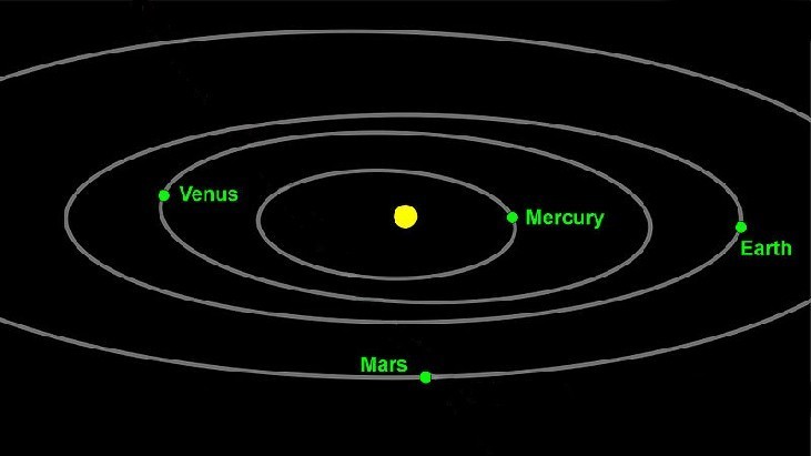
Figure 1. Planets follow elliptical paths as they orbit around the Sun. (credit: modification of work by NASA/JPL-Caltech)
The planets move through space in elliptical, periodic orbits about the sun, as shown in Figure 1. They are in constant motion, so fixing an exact position of any planet is valid only for a moment. In other words, we can fix only a planet’s instantaneous position. This is one application of polar coordinates, represented as [latex]\left(r,\theta \right)[/latex]. We interpret [latex]r[/latex] as the distance from the sun and [latex]\theta[/latex] as the planet’s angular bearing, or its direction from a fixed point on the sun. In this section, we will focus on the polar system and the graphs that are generated directly from polar coordinates.
Testing Polar Equations for Symmetry
Just as a rectangular equation such as [latex]y={x}^{2}[/latex] describes the relationship between [latex]x[/latex] and [latex]y[/latex] on a Cartesian grid, a polar equation describes a relationship between [latex]r[/latex] and [latex]\theta[/latex] on a polar grid. Recall that the coordinate pair [latex]\left(r,\theta \right)[/latex] indicates that we move counterclockwise from the polar axis (positive x-axis) by an angle of [latex]\theta[/latex], and extend a ray from the pole (origin) [latex]r[/latex] units in the direction of [latex]\theta[/latex]. All points that satisfy the polar equation are on the graph.
Symmetry is a property that helps us recognize and plot the graph of any equation. If an equation has a graph that is symmetric with respect to an axis, it means that if we folded the graph in half over that axis, the portion of the graph on one side would coincide with the portion on the other side. By performing three tests, we will see how to apply the properties of symmetry to polar equations. Further, we will use symmetry (in addition to plotting key points, zeros, and maximums of [latex]r[/latex])
to determine the graph of a polar equation.
In the first test, we consider symmetry with respect to the line [latex]\theta =\frac{\pi }{2}[/latex] (y-axis). We replace [latex]\left(r,\theta \right)[/latex] with [latex]\left(-r,-\theta \right)[/latex] to determine if the new equation is equivalent to the original equation. For example, suppose we are given the equation [latex]r=2\sin \theta[/latex];
This equation exhibits symmetry with respect to the line [latex]\theta =\frac{\pi }{2}[/latex].
In the second test, we consider symmetry with respect to the polar axis ( [latex]x[/latex] -axis). We replace [latex]\left(r,\theta \right)[/latex] with [latex]\left(r,-\theta \right)[/latex] or [latex]\left(-r,\pi -\theta \right)[/latex] to determine equivalency between the tested equation and the original. For example, suppose we are given the equation [latex]r=1 - 2\cos \theta[/latex].
The graph of this equation exhibits symmetry with respect to the polar axis.
In the third test, we consider symmetry with respect to the pole (origin). We replace [latex]\left(r,\theta \right)[/latex] with [latex]\left(-r,\theta \right)[/latex] to determine if the tested equation is equivalent to the original equation. For example, suppose we are given the equation [latex]r=2\sin \left(3\theta \right)[/latex].
The equation has failed the symmetry test, but that does not mean that it is not symmetric with respect to the pole. Passing one or more of the symmetry tests verifies that symmetry will be exhibited in a graph. However, failing the symmetry tests does not necessarily indicate that a graph will not be symmetric about the line [latex]\theta =\frac{\pi }{2}[/latex], the polar axis, or the pole. In these instances, we can confirm that symmetry exists by plotting reflecting points across the apparent axis of symmetry or the pole. Testing for symmetry is a technique that simplifies the graphing of polar equations, but its application is not perfect.
A General Note: Symmetry Tests
A polar equation describes a curve on the polar grid. The graph of a polar equation can be evaluated for three types of symmetry, as shown in Figure 2.
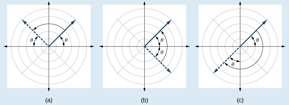
Figure 2. (a) A graph is symmetric with respect to the line [latex]\theta =\frac{\pi }{2}[/latex] (y-axis) if replacing [latex]\left(r,\theta \right)[/latex] with [latex]\left(-r,-\theta \right)[/latex] yields an equivalent equation. (b) A graph is symmetric with respect to the polar axis (x-axis) if replacing [latex]\left(r,\theta \right)[/latex] with [latex]\left(r,-\theta \right)[/latex] or [latex]\left(-r,\mathrm{\pi -}\theta \right)[/latex] yields an equivalent equation. (c) A graph is symmetric with respect to the pole (origin) if replacing [latex]\left(r,\theta \right)[/latex] with [latex]\left(-r,\theta \right)[/latex] yields an equivalent equation.
How To: Given a polar equation, test for symmetry.
- Substitute the appropriate combination of components for [latex]\left(r,\theta \right):[/latex] [latex]\left(-r,-\theta \right)[/latex] for [latex]\theta =\frac{\pi }{2}[/latex] symmetry; [latex]\left(r,-\theta \right)[/latex] for polar axis symmetry; and [latex]\left(-r,\theta \right)[/latex] for symmetry with respect to the pole.
- If the resulting equations are equivalent in one or more of the tests, the graph produces the expected symmetry.
Example 1: Testing a Polar Equation for Symmetry
Test the equation [latex]r=2\sin \theta[/latex] for symmetry.

Try It
Test the equation for symmetry: [latex]r=-2\cos \theta[/latex].
Try It
Graphing Polar Equations by Plotting Points
To graph in the rectangular coordinate system we construct a table of [latex]x[/latex] and [latex]y[/latex] values. To graph in the polar coordinate system we construct a table of [latex]\theta[/latex] and [latex]r[/latex] values. We enter values of [latex]\theta[/latex] into a polar equation and calculate [latex]r[/latex]. However, using the properties of symmetry and finding key values of [latex]\theta[/latex] and [latex]r[/latex] means fewer calculations will be needed.
Finding Zeros and Maxima
To find the zeros of a polar equation, we solve for the values of [latex]\theta[/latex] that result in [latex]r=0[/latex]. Recall that, to find the zeros of polynomial functions, we set the equation equal to zero and then solve for [latex]x[/latex]. We use the same process for polar equations. Set [latex]r=0[/latex], and solve for [latex]\theta[/latex].
For many of the forms we will encounter, the maximum value of a polar equation is found by substituting those values of [latex]\theta[/latex] into the equation that result in the maximum value of the trigonometric functions. Consider [latex]r=5\cos \theta[/latex]; the maximum distance between the curve and the pole is 5 units. The maximum value of the cosine function is 1 when [latex]\theta =0[/latex], so our polar equation is [latex]5\cos \theta[/latex], and the value [latex]\theta =0[/latex] will yield the maximum [latex]|r|[/latex].
Similarly, the maximum value of the sine function is 1 when [latex]\theta =\frac{\pi }{2}[/latex], and if our polar equation is [latex]r=5\sin \theta[/latex], the value [latex]\theta =\frac{\pi }{2}[/latex] will yield the maximum [latex]|r|[/latex]. We may find additional information by calculating values of [latex]r[/latex] when [latex]\theta =0[/latex]. These points would be polar axis intercepts, which may be helpful in drawing the graph and identifying the curve of a polar equation.
Example 2: Finding Zeros and Maximum Values for a Polar Equation
Using the equation in Example 1, find the zeros and maximum [latex]|r|[/latex] and, if necessary, the polar axis intercepts of [latex]r=2\sin \theta[/latex].

Try It
Without converting to Cartesian coordinates, test the given equation for symmetry and find the zeros and maximum values of [latex]|r|:[/latex] [latex]r=3\cos \theta[/latex].
Graphing Circles and the 5 Classic Polar Curves
Investigating Circles
Now we have seen the equation of a circle in the polar coordinate system. In the last two examples, the same equation was used to illustrate the properties of symmetry and demonstrate how to find the zeros, maximum values, and plotted points that produced the graphs. However, the circle is only one of many shapes in the set of polar curves.
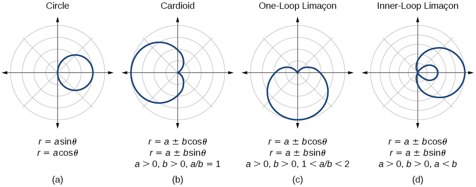
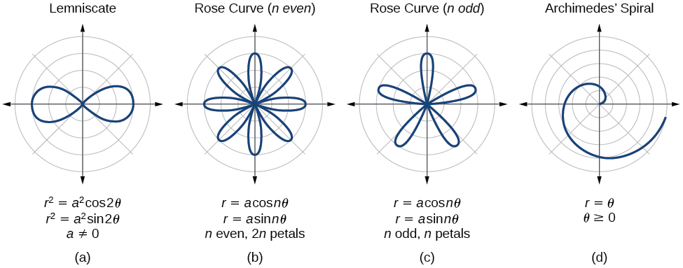
There are five classic polar curves: cardioids, limaҫons, lemniscates, rose curves, and Archimedes’ spirals. We will briefly touch on the polar formulas for the circle before moving on to the classic curves and their variations.
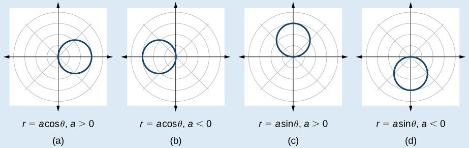
A General Note: Formulas for the Equation of a Circle
Some of the formulas that produce the graph of a circle in polar coordinates are given by [latex]r=a\cos \theta[/latex] and [latex]r=a\sin \theta[/latex], where [latex]a[/latex] is the diameter of the circle or the distance from the pole to the farthest point on the circumference. The radius is [latex]\frac{|a|}{2}[/latex], or one-half the diameter. For [latex]r=a\cos \theta ,[/latex] the center is [latex]\left(\frac{a}{2},0\right)[/latex]. For [latex]r=a\sin \theta[/latex], the center is [latex]\left(\frac{a}{2},\pi \right)[/latex]. Figure 5 shows the graphs of these four circles.
Example 3: Sketching the Graph of a Polar Equation for a Circle
Sketch the graph of [latex]r=4\cos \theta[/latex].

Investigating Cardioids
While translating from polar coordinates to Cartesian coordinates may seem simpler in some instances, graphing the classic curves is actually less complicated in the polar system. The next curve is called a cardioid, as it resembles a heart. This shape is often included with the family of curves called limaçons, but here we will discuss the cardioid on its own.
A General Note: Formulas for a Cardioid
The formulas that produce the graphs of a cardioid are given by [latex]r=a\pm b\cos \theta[/latex] and [latex]r=a\pm b\sin \theta[/latex] where [latex]a>0,b>0[/latex], and [latex]\frac{a}{b}=1[/latex]. The cardioid graph passes through the pole, as we can see in Figure 7.
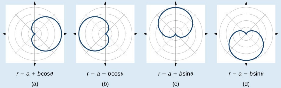
Figure 7
How To: Given the polar equation of a cardioid, sketch its graph.
- Check equation for the three types of symmetry.
- Find the zeros. Set [latex]r=0[/latex].
- Find the maximum value of the equation according to the maximum value of the trigonometric expression.
- Make a table of values for [latex]r[/latex] and [latex]\theta[/latex].
- Plot the points and sketch the graph.
Example 4: Sketching the Graph of a Cardioid
Sketch the graph of [latex]r=2+2\cos \theta[/latex].

Investigating Limaçons
The word limaçon is Old French for “snail,” a name that describes the shape of the graph. As mentioned earlier, the cardioid is a member of the limaçon family, and we can see the similarities in the graphs. The other images in this category include the one-loop limaçon and the two-loop (or inner-loop) limaçon. One-loop limaçons are sometimes referred to as dimpled limaçons when [latex]1<\frac{a}{b}<2[/latex] and convex limaçons when [latex]\frac{a}{b}\ge 2[/latex].
A General Note: Formulas for One-Loop Limaçons
The formulas that produce the graph of a dimpled one-loop limaçon are given by [latex]r=a\pm b\cos \theta[/latex] and [latex]r=a\pm b\sin \theta[/latex] where [latex]a>0,b>0,\text{and 1<}\frac{a}{b}<2[/latex]. All four graphs are shown in Figure 9.
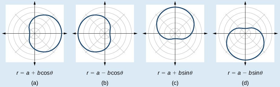
Figure 9. Dimpled limaçons
How To: Given a polar equation for a one-loop limaçon, sketch the graph.
- Test the equation for symmetry. Remember that failing a symmetry test does not mean that the shape will not exhibit symmetry. Often the symmetry may reveal itself when the points are plotted.
- Find the zeros.
- Find the maximum values according to the trigonometric expression.
- Make a table.
- Plot the points and sketch the graph.
Example 5: Sketching the Graph of a One-Loop Limaçon
Graph the equation [latex]r=4 - 3\sin \theta[/latex].

Try It
Sketch the graph of [latex]r=3 - 2\cos \theta[/latex].

Try It
Another type of limaçon, the inner-loop limaçon, is named for the loop formed inside the general limaçon shape. It was discovered by the German artist Albrecht Dürer(1471-1528), who revealed a method for drawing the inner-loop limaçon in his 1525 book Underweysung der Messing. A century later, the father of mathematician Blaise Pascal, Étienne Pascal(1588-1651), rediscovered it.
A General Note: Formulas for Inner-Loop Limaçons
The formulas that generate the inner-loop limaçons are given by [latex]r=a\pm b\cos \theta[/latex] and [latex]r=a\pm b\sin \theta[/latex] where [latex]a>0,b>0[/latex], and [latex]a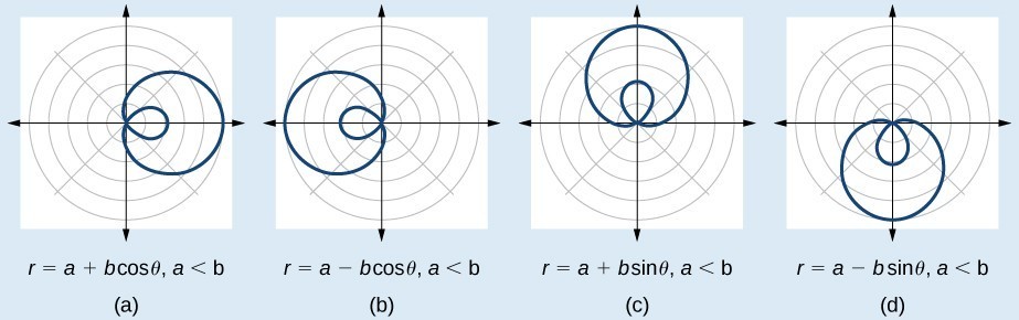
Figure 11


![Two graphs side by side of Archimedes' spiral. (A) is r= theta, [0, 2pi]. (B) is r=theta, [0, 4pi]. Both start at origin and spiral out counterclockwise. The second has two spirals out while the first has one.](https://s3-us-west-2.amazonaws.com/courses-images/wp-content/uploads/sites/3675/2018/09/27165546/CNX_Precalc_Figure_08_04_020new.jpg)
![Graph of Archimedes' spiral r=theta over [0,2pi]. Starts at origin and spirals out in one loop counterclockwise. Points (pi/4, pi/4), (pi/2,pi/2), (pi,pi), (5pi/4, 5pi/4), (7pi/4, pi/4), and (2pi, 2pi) are marked.](https://s3-us-west-2.amazonaws.com/courses-images/wp-content/uploads/sites/3675/2018/09/27165549/CNX_Precalc_Figure_08_04_021F.jpg)