Learning Outcomes
- Find the average rate of change of a function.
- Use a graph to determine where a function is increasing, decreasing, or constant.
- Use a graph to locate local and absolute maxima and local minima.
Gasoline costs have experienced some wild fluctuations over the last several decades. The table below[1] lists the average cost, in dollars, of a gallon of gasoline for the years 2005–2012. The cost of gasoline can be considered as a function of year.
| [latex]y[/latex] | 2005 | 2006 | 2007 | 2008 | 2009 | 2010 | 2011 | 2012 |
| [latex]C\left(y\right)[/latex] | 2.31 | 2.62 | 2.84 | 3.30 | 2.41 | 2.84 | 3.58 | 3.68 |
If we were interested only in how the gasoline prices changed between 2005 and 2012, we could compute that the cost per gallon had increased from $2.31 to $3.68, an increase of $1.37. While this is interesting, it might be more useful to look at how much the price changed per year. In this section, we will investigate changes such as these.
Finding the Average Rate of Change of a Function
The price change per year is a rate of change because it describes how an output quantity changes relative to the change in the input quantity. We can see that the price of gasoline in the table above did not change by the same amount each year, so the rate of change was not constant. If we use only the beginning and ending data, we would be finding the average rate of change over the specified period of time. To find the average rate of change, we divide the change in the output value by the change in the input value.
The Greek letter [latex]\Delta[/latex] (delta) signifies the change in a quantity; we read the ratio as “delta-y over delta-x” or “the change in [latex]y[/latex] divided by the change in [latex]x[/latex].” Occasionally we write [latex]\Delta f[/latex] instead of [latex]\Delta y[/latex], which still represents the change in the function’s output value resulting from a change to its input value. It does not mean we are changing the function into some other function.
In our example, the gasoline price increased by $1.37 from 2005 to 2012. Over 7 years, the average rate of change was
On average, the price of gas increased by about 19.6¢ each year.
Other examples of rates of change include:
- A population of rats increasing by 40 rats per week
- A car traveling 68 miles per hour (distance traveled changes by 68 miles each hour as time passes)
- A car driving 27 miles per gallon (distance traveled changes by 27 miles for each gallon)
- The current through an electrical circuit increasing by 0.125 amperes for every volt of increased voltage
- The amount of money in a college account decreasing by $4,000 per quarter
A General Note: Rate of Change
A rate of change describes how an output quantity changes relative to the change in the input quantity. The units on a rate of change are “output units per input units.”
The average rate of change between two input values is the total change of the function values (output values) divided by the change in the input values.
How To: Given the value of a function at different points, calculate the average rate of change of a function for the interval between two values [latex]{x}_{1}[/latex] and [latex]{x}_{2}[/latex].
- Calculate the difference [latex]{y}_{2}-{y}_{1}=\Delta y[/latex].
- Calculate the difference [latex]{x}_{2}-{x}_{1}=\Delta x[/latex].
- Find the ratio [latex]\frac{\Delta y}{\Delta x}[/latex].
Example 1: Computing an Average Rate of Change
Using the data in the table below, find the average rate of change of the price of gasoline between 2007 and 2009.
| [latex]y[/latex] | 2005 | 2006 | 2007 | 2008 | 2009 | 2010 | 2011 | 2012 |
| [latex]C\left(y\right)[/latex] | 2.31 | 2.62 | 2.84 | 3.30 | 2.41 | 2.84 | 3.58 | 3.68 |
The following video provides another example of how to find the average rate of change between two points from a table of values.
Try It
Using the data in the table below, find the average rate of change between 2005 and 2010.
| [latex]y[/latex] | 2005 | 2006 | 2007 | 2008 | 2009 | 2010 | 2011 | 2012 |
| [latex]C\left(y\right)[/latex] | 2.31 | 2.62 | 2.84 | 3.30 | 2.41 | 2.84 | 3.58 | 3.68 |
Example 2: Computing Average Rate of Change from a Graph
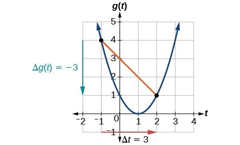
Given the function [latex]g\left(t\right)[/latex] shown in Figure 1, find the average rate of change on the interval [latex]\left[-1,2\right][/latex].
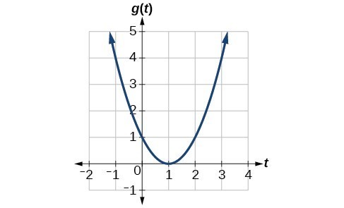
Figure 1
Example 3: Computing Average Rate of Change from a Table
After picking up a friend who lives 10 miles away, Anna records her distance from home over time. The values are shown in the table below. Find her average speed over the first 6 hours.
| t (hours) | 0 | 1 | 2 | 3 | 4 | 5 | 6 | 7 |
| D(t) (miles) | 10 | 55 | 90 | 153 | 214 | 240 | 292 | 300 |
Example 4: Computing Average Rate of Change for a Function Expressed as a Formula
Compute the average rate of change of [latex]f\left(x\right)={x}^{2}-\frac{1}{x}[/latex] on the interval [latex]\text{[2,}\text{4].}[/latex]
The following video provides another example of finding the average rate of change of a function given a formula and an interval.
Try It
Find the average rate of change of [latex]f\left(x\right)=x - 2\sqrt{x}[/latex] on the interval [latex]\left[1,9\right][/latex].
Try It
Example 5: Finding the Average Rate of Change of a Force
The electrostatic force [latex]F[/latex], measured in newtons, between two charged particles can be related to the distance between the particles [latex]d[/latex], in centimeters, by the formula [latex]F\left(d\right)=\frac{2}{{d}^{2}}[/latex]. Find the average rate of change of force if the distance between the particles is increased from 2 cm to 6 cm.
Example 6: Finding an Average Rate of Change as an Expression
Find the average rate of change of [latex]g\left(t\right)={t}^{2}+3t+1[/latex] on the interval [latex]\left[0,a\right][/latex]. The answer will be an expression involving [latex]a[/latex].
Try It
Find the average rate of change of [latex]f\left(x\right)={x}^{2}+2x - 8[/latex] on the interval [latex]\left[5,a\right][/latex].
As part of exploring how functions change, we can identify intervals over which the function is changing in specific ways. We say that a function is increasing on an interval if the function values increase as the input values increase within that interval. Similarly, a function is decreasing on an interval if the function values decrease as the input values increase over that interval. The average rate of change of an increasing function is positive, and the average rate of change of a decreasing function is negative. Figure 3 shows examples of increasing and decreasing intervals on a function.
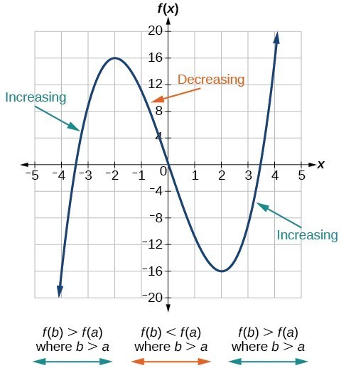
Figure 3. The function [latex]f\left(x\right)={x}^{3}-12x[/latex] is increasing on [latex]\left(-\infty \text{,}-\text{2}\right){{\cup }^{\text{ }}}^{\text{ }}\left(2,\infty \right)[/latex] and is decreasing on [latex]\left(-2\text{,}2\right)[/latex].
This video further explains how to find where a function is increasing or decreasing.
While some functions are increasing (or decreasing) over their entire domain, many others are not. A value of the input where a function changes from increasing to decreasing (as we go from left to right, that is, as the input variable increases) is called a local maximum. If a function has more than one, we say it has local maxima. Similarly, a value of the input where a function changes from decreasing to increasing as the input variable increases is called a local minimum. The plural form is “local minima.” Together, local maxima and minima are called local extrema, or local extreme values, of the function. (The singular form is “extremum.”) Often, the term local is replaced by the term relative. In this text, we will use the term local.
Clearly, a function is neither increasing nor decreasing on an interval where it is constant. A function is also neither increasing nor decreasing at extrema. Note that we have to speak of local extrema, because any given local extremum as defined here is not necessarily the highest maximum or lowest minimum in the function’s entire domain.
For the function in Figure 4, the local maximum is 16, and it occurs at [latex]x=-2[/latex]. The local minimum is [latex]-16[/latex] and it occurs at [latex]x=2[/latex].
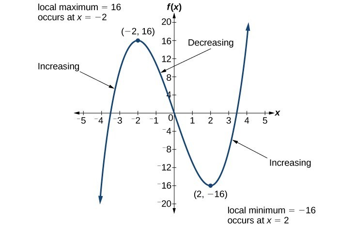
Figure 4
To locate the local maxima and minima from a graph, we need to observe the graph to determine where the graph attains its highest and lowest points, respectively, within an open interval. Like the summit of a roller coaster, the graph of a function is higher at a local maximum than at nearby points on both sides. The graph will also be lower at a local minimum than at neighboring points. Figure 5 illustrates these ideas for a local maximum.
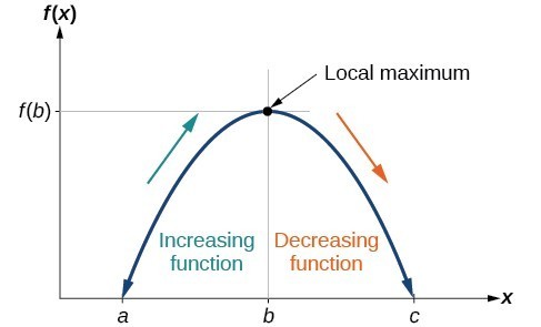
Figure 5. Definition of a local maximum.
These observations lead us to a formal definition of local extrema.
A General Note: Local Minima and Local Maxima
A function [latex]f[/latex] is an increasing function on an open interval if [latex]f\left(b\right)>f\left(a\right)[/latex] for any two input values [latex]a[/latex] and [latex]b[/latex] in the given interval where [latex]b>a[/latex].
A function [latex]f[/latex] is a decreasing function on an open interval if [latex]f\left(b\right)
A function [latex]f[/latex] has a local maximum at [latex]x=b[/latex] if there exists an interval [latex]\left(a,c\right)[/latex] with [latex]a
Example 7: Finding Increasing and Decreasing Intervals on a Graph
Given the function [latex]p\left(t\right)[/latex] in the graph below, identify the intervals on which the function appears to be increasing.
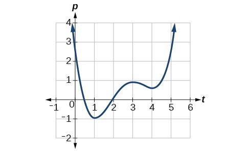
Figure 6
Example 8: Finding Local Extrema from a Graph
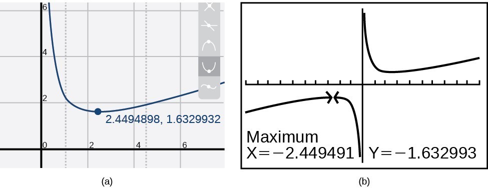
Graph the function [latex]f\left(x\right)=\frac{2}{x}+\frac{x}{3}[/latex]. Then use the graph to estimate the local extrema of the function and to determine the intervals on which the function is increasing.
Try It
Graph the function [latex]f\left(x\right)={x}^{3}-6{x}^{2}-15x+20[/latex] to estimate the local extrema of the function. Use these to determine the intervals on which the function is increasing and decreasing.

Try It
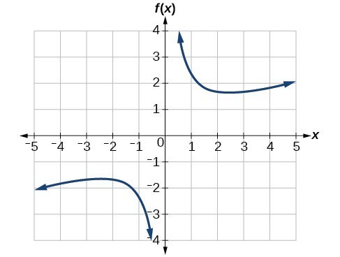
Example 9: Finding Local Maxima and Minima from a Graph
For the function [latex]f[/latex] whose graph is shown in Figure 9, find all local maxima and minima.
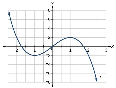
Figure 9
Analyzing the Toolkit Functions for Increasing or Decreasing Intervals
We will now return to our toolkit functions and discuss their graphical behavior in the table below.
| Function | Increasing/Decreasing | Example |
|---|---|---|
| Constant Function
[latex]f\left(x\right)={c}[/latex] |
Neither increasing nor decreasing | 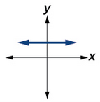 |
| Identity Function
[latex]f\left(x\right)={x}[/latex] |
Increasing | 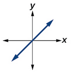 |
| Quadratic Function
[latex]f\left(x\right)={x}^{2}[/latex] |
Increasing on [latex]\left(0,\infty\right)[/latex]
Decreasing on [latex]\left(-\infty,0\right)[/latex] Minimum at [latex]x=0[/latex] |
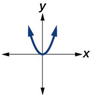 |
| Cubic Function
[latex]f\left(x\right)={x}^{3}[/latex] |
Increasing |  |
| Reciprocal
[latex]f\left(x\right)=\frac{1}{x}[/latex] |
Decreasing [latex]\left(-\infty,0\right)\cup\left(0,\infty\right)[/latex] |  |
| Reciprocal Squared
[latex]f\left(x\right)=\frac{1}{{x}^{2}}[/latex] |
Increasing on [latex]\left(-\infty,0\right)[/latex]
Decreasing on [latex]\left(0,\infty\right)[/latex] |
 |
| Cube Root
[latex]f\left(x\right)=\sqrt[3]{x}[/latex]
|
Increasing |  |
| Square Root
[latex]f\left(x\right)=\sqrt{x}[/latex] |
Increasing on [latex]\left(0,\infty\right)[/latex] | 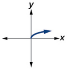 |
| Absolute Value
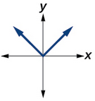
[latex]f\left(x\right)=|x|[/latex] |
Increasing on [latex]\left(0,\infty\right)[/latex]
Decreasing on [latex]\left(-\infty,0\right)[/latex] |
 |
Use A Graph to Locate the Absolute Maximum and Absolute Minimum
There is a difference between locating the highest and lowest points on a graph in a region around an open interval (locally) and locating the highest and lowest points on the graph for the entire domain. The [latex]y\text{-}[/latex] coordinates (output) at the highest and lowest points are called the absolute maximum and absolute minimum, respectively.
To locate absolute maxima and minima from a graph, we need to observe the graph to determine where the graph attains it highest and lowest points on the domain of the function. See Figure 10.
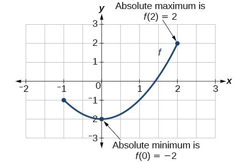
Figure 10
Not every function has an absolute maximum or minimum value. The toolkit function [latex]f\left(x\right)={x}^{3}[/latex] is one such function.
A General Note: Absolute Maxima and Minima
The absolute maximum of [latex]f[/latex] at [latex]x=c[/latex] is [latex]f\left(c\right)[/latex] where [latex]f\left(c\right)\ge f\left(x\right)[/latex] for all [latex]x[/latex] in the domain of [latex]f[/latex].
The absolute minimum of [latex]f[/latex] at [latex]x=d[/latex] is [latex]f\left(d\right)[/latex] where [latex]f\left(d\right)\le f\left(x\right)[/latex] for all [latex]x[/latex] in the domain of [latex]f[/latex].
Example 10: Finding Absolute Maxima and Minima from a Graph
For the function [latex]f[/latex] shown in Figure 11, find all absolute maxima and minima.
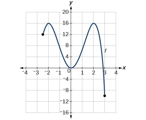
Figure 11
Key Equations
| Average rate of change | [latex]\dfrac{\Delta y}{\Delta x}=\dfrac{f\left({x}_{2}\right)-f\left({x}_{1}\right)}{{x}_{2}-{x}_{1}}[/latex] |
Key Concepts
- A rate of change relates a change in an output quantity to a change in an input quantity. The average rate of change is determined using only the beginning and ending data.
- Identifying points that mark the interval on a graph can be used to find the average rate of change.
- Comparing pairs of input and output values in a table can also be used to find the average rate of change.
- An average rate of change can also be computed by determining the function values at the endpoints of an interval described by a formula.
- The average rate of change can sometimes be determined as an expression.
- A function is increasing where its rate of change is positive and decreasing where its rate of change is negative.
- A local maximum is where a function changes from increasing to decreasing and has an output value larger (more positive or less negative) than output values at neighboring input values.
- A local minimum is where the function changes from decreasing to increasing (as the input increases) and has an output value smaller (more negative or less positive) than output values at neighboring input values.
- Minima and maxima are also called extrema.
- We can find local extrema from a graph.
- The highest and lowest points on a graph indicate the maxima and minima.
Glossary
- absolute maximum
- the greatest value of a function over an interval
- absolute minimum
- the lowest value of a function over an interval
- average rate of change
- the difference in the output values of a function found for two values of the input divided by the difference between the inputs
- decreasing function
- a function is decreasing in some open interval if [latex]f\left(b\right)
- increasing function
- a function is increasing in some open interval if [latex]f\left(b\right)>f\left(a\right)[/latex] for any two input values [latex]a[/latex] and [latex]b[/latex] in the given interval where [latex]b>a[/latex]
- local extrema
- collectively, all of a function’s local maxima and minima
- local maximum
- a value of the input where a function changes from increasing to decreasing as the input value increases.
- local minimum
- a value of the input where a function changes from decreasing to increasing as the input value increases.
- rate of change
- the change of an output quantity relative to the change of the input quantity
Candela Citations
- Precalculus. Authored by: OpenStax College. Provided by: OpenStax. Located at: http://cnx.org/contents/fd53eae1-fa23-47c7-bb1b-972349835c3c@5.175:1/Preface. License: CC BY: Attribution
- http://www.eia.gov/totalenergy/data/annual/showtext.cfm?t=ptb0524. Accessed 3/5/2014. ↵