A linear inequality is the same as a linear equation [latex]Ax+By=C,[/latex] but with the equal sign replaced with an inequality sign. An example is [latex]2x-3y\leq4.[/latex] Often a linear inequality is written in “slope-intercept form,” for example [latex]y\leq x-2.[/latex]

An ordered pair is a solution if it makes the inequality true when we substitute [latex]x[/latex] and [latex]y.[/latex] Here is a quick example.

It is not a useful strategy to find all solutions to a linear inequality by testing single ordered pairs. We will see that linear inequalities have infinitely many solutions, so a graph in the coordinate plane is a good way to represent the solution set.

Let’s consider a first example, to graph the inequality

[latex]x+4y\leq4[/latex].

Any point on the line [latex]x+4y=4[/latex] will satisfy the inequality since this inequality symbol allows equality, so we begin by graphing the line. You can use the [latex]x[/latex] and [latex]y[/latex]-intercepts for this equation to graph the line. For example, find the [latex]y[/latex]-intercept by setting [latex]x=0[/latex] and solving for [latex]y.[/latex]

Plot the points [latex](0,1)[/latex] and [latex](4,0)[/latex], and draw a line through these two points. This line is called the boundary line.

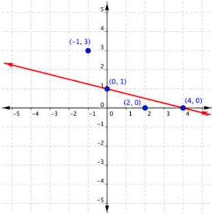
Next, let’s test a couple of ordered pairs, one on each side of the boundary line.

If you substitute [latex](−1,3)[/latex] into [latex]x+4y\leq4[/latex]:

[latex]\begin{array}{r}−1+4\left(3\right)\overset{?}{\leq}4\\−1+12\overset{?}{\leq}4\\11\not\leq4\end{array}[/latex]

This is a false statement so [latex](−1,3)[/latex] is not a solution.

On the other hand, if you substitute [latex](2,0)[/latex] into [latex]x+4y\leq4[/latex]:

[latex]\begin{array}{r}2+4\left(0\right)\overset{?}{\leq}4\\2+0\overset{?}{\leq}4\\2\leq4\end{array}[/latex]

This is true! As it turns out, the boundary line is the dividing line between solutions and non-solutions. We call each side of the line a half-plane. The half-plane that includes [latex](2,0)[/latex] should be shaded to indicate this is the region of solutions for the inequality. The half-plane that includes [latex](-1,3)[/latex] has no solutions.

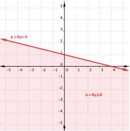
And there you have it, the graph of the set of solutions for [latex]x+4y\leq4[/latex]. Here is our process in summarized form.

Below is a video about how to graph inequalities with two variables.

Example

Graph the inequality [latex]2y>4x–6[/latex].

Show Solution

First we need to graph the boundary line. In this example we can do this by writing it in slope intercept form. Remember to switch the inequality sign if dividing by a negative number during this step.

[latex] \displaystyle \begin{array}{rl}2y&>\; 4x-6\\\\\dfrac{2y}{2}&>\; \dfrac{4x}{2}-\dfrac{6}{2}\\\\y&>\; 2x-3\\\end{array}[/latex]

Create a table of values to find two points on the line [latex] \displaystyle y=2x-3.[/latex]

[latex]x[/latex]	[latex]y[/latex]
[latex]0[/latex]	[latex]-3[/latex]
[latex]2[/latex]	[latex]1[/latex]

Plot the points and graph the line. The line is dashed because the sign in the inequality is [latex]>[/latex], not [latex]\geq[/latex] and therefore points on the line are not solutions to the inequality.

An ordered pair on each side of the boundary line is chosen above. Test each point in the original inequality.

[latex]\begin{array}{l}\\\text{Test }1:\left(−3,1\right)\\2\left(1\right)\overset{?}{>}4\left(−3\right)–6\\\,\,\,\,\,\,\,2\overset{?}{>}–12–6\\\,\,\,\,\,\,\,2>−18\\\,\,\,\,\,\,\,\,\text{TRUE}\\\\\text{Test }2:\left(4,1\right)\\2(1)\overset{?}{>}4\left(4\right)– 6\\\,\,\,\,\,\,2\overset{?}{>}16–6\\\,\,\,\,\,\,2\not >10\\\,\,\,\,\,\text{FALSE}\end{array}[/latex]

Since [latex](−3,1)[/latex] results in a true statement, the half-plane that includes [latex](−3,1)[/latex] should be shaded.

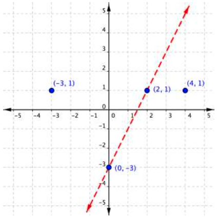
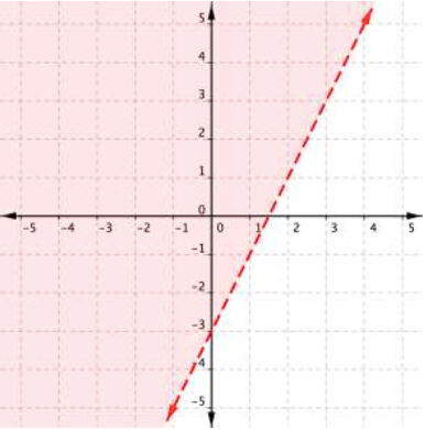
The graph of the inequality [latex]2y>4x–6[/latex] is:

Note that you can use the points [latex](0,−3)[/latex] and [latex](2,1)[/latex] to graph the boundary line, but these points are not included in the region of solutions since the region does not include the boundary line!

Also note that we only really needed to use one test point instead of two, since we know only one side of the line can be the solution region. If the first test point results in a false statement, shade the other side.

If you rewrite your inequality in slope-intercept form as in the previous example, it provides an alternative approach to deciding the direction of shading. A [latex]>[/latex] or [latex]\geq[/latex] symbol as we had in that example always means shade above the line. A [latex]<[/latex] or [latex]\leq[/latex] symbol means shade below. Note this approach does not work unless the inequality is put into slope-intercept form!

This video gives an example of using this alternative approach to do the shading.

Systems of Two or More Inequalities

The graph of a single linear inequality in two variables splits the coordinate plane into two regions. On one side lie all the solutions to the inequality. Now consider the system of inequalities,

[latex]\left\{ \begin{array}{l}y<2x+5\\y>-x \end{array} \right.[/latex]

Here are the graphs of each inequality independently.

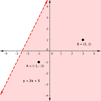
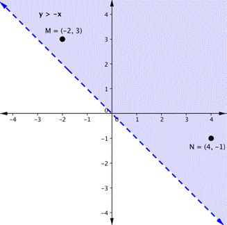
You can verify by substitution that points [latex]A[/latex] and [latex]B[/latex] satisfy the first inequality, while points [latex]M[/latex] and [latex]N[/latex] satisfy the second inequality.

A solution to a system of inequalities must satisfy both inequalities at the same time. The solution set consists of all points which satisfy both inequalities. The easiest way to find the solution set is to graph both inequalities on the same graph and find the region of overlap.

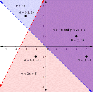
The purple area shows where the solutions of the two inequalities overlap. This area is the solution to the system of inequalities. Any point within this purple region will be true for both [latex]y<2x+5[/latex] and [latex]y>−x.[/latex] Note in particular that the blue and red regions do NOT solve the system because they only satisfy one of the two inequalities. In the future, we will usually only shade the overlap region to avoid confusion.

We can verify by substitution that the point [latex]M=(-2,3)[/latex] in the blue region is not a solution to the system since it does not satisfy the first inequality:

[latex]\begin{align}y&<2x+5\\ 3&<2(-2)+5\\ 3&<-4+5\\ 3&<1&&\color{red}{\textsf{False}}\end{align}[/latex]

In the following video examples, we show how to graph a system of linear inequalities and define the solution region.

The general steps are outlined below.

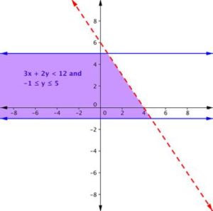
The system in our next example includes a compound inequality.  We will see that you can treat a compound inequality like two inequalities when you are graphing them, so this example is basically a system of three inequalities.

Example

Graph the system

[latex]\left\{ \begin{array}{rl}3x+2y&<12\\-1 \leq y &\leq 5 \end{array} \right.[/latex]

Show Solution

Begin by graphing the first inequality. The boundary line has intercepts at [latex](0,6)[/latex] and [latex](4,0)[/latex] and the line should be dashed. Testing the point [latex](0,0)[/latex] will show that the area below the line is the solution to this inequality.

The inequality [latex] -1 ≤ y ≤ 5[/latex] is actually two inequalities: [latex]−1 ≤ y,[/latex] and [latex]y ≤ 5.[/latex] Another way to think of this is [latex]y[/latex] must be between [latex]−1[/latex] and [latex]5[/latex]. The border lines for both are horizontal. The region between those two lines contains the solutions of [latex] -1 ≤ y ≤ 5[/latex]. We make the lines solid because we also want to include [latex]y = −1[/latex] and [latex]y=5[/latex].

Graph this region on the same axes as the other inequality.

The purple region shows the set of all solutions of the system.

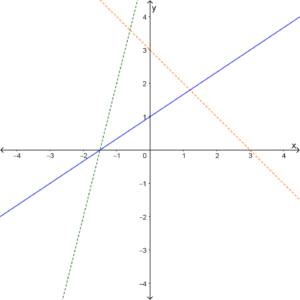
The next example is explicitly a system of three inequalities to graph.

EXAMPLE

Graph the system

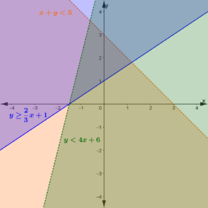
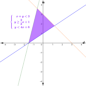
[latex]\left\{ \begin{array}{rl}x+y<3\\y\geq\dfrac{2}{3}x+1\\y<4x+6 \end{array} \right.[/latex]

Show Solution

Begin by graphing all three boundary lines on the same axes. This splits the plane into seven regions. Only one of them can be the solution region.

The point [latex](0,0)[/latex] is not on any of the lines, so use it as a test point.

Inequality 1 (red):  [latex]0+0\leq 3[/latex] TRUE

Inequality 2 (blue):  [latex]0\geq \dfrac{2}{3}\cdot 0 + 1, \textsf{ or } 0 \geq 1[/latex] FALSE

Inequality 3 (green):  [latex]0<4\cdot 0 + 6, \textsf{ or } 0<6[/latex] TRUE

For lines 1 (red) and 3 (green) we shade toward the point [latex](0, 0),[/latex] which means down. For line 2 (blue) we shade away from the point [latex](0,0),[/latex] which means up.

The solution region is the one shaded all three times, which is the center triangle. If we want to be extra sure, we can test another point which is inside that triangle and verify that it satisfies all three inequalities. Test point [latex](0,2):[/latex]

Inequality 1:  [latex]0+2\leq 3[/latex] TRUE

Inequality 2:  [latex]2\geq \dfrac{2}{3}\cdot 0 + 1, \textsf{ or } 2 \geq 1[/latex] TRUE

Inequality 3:  [latex]2<4\cdot 0 + 6, \textsf{ or } 2<6[/latex] TRUE

The solution region is the center triangle. Two edges of the triangle are dashed (not solutions), and the bottom edge which is part of the blue line is in the solution set.

Note that by modifying the original problem and switching the direction of some of the inequality symbols, we could have made any of the seven regions be the solution region. For example, switching only Inequality 2 to a [latex]\leq[/latex] sign would have caused our first test point [latex](0,0)[/latex] to satisfy all three inequalities, so the solution region would have been the bottom, unbounded region containing [latex](0,0).[/latex]

Summary

When linear inequalities are graphed on a coordinate plane, the solution takes the form of all points on one side of the boundary line, and possibly also the line itself. You can tell which region to shade by testing some points in the inequality, or observing the direction of the sign if the inequality is in slope-intercept form. When graphing a system of linear inequalities, graph all inequalities on the same axes. The solution set is the overlap of all the individual solution sets.