A graph is more than just an image; it’s a powerful tool for visually representing the precise relationship between two variables. Mastering the ability to interpret and create graphs is a vital skill that you’ll carry into your chosen field and beyond, enhancing your understanding and communication in both your professional and civic life.

Mathematics is a crucial tool for making sense of the world around us. Whether you’re a scientist, social scientist, engineer, business leader, health care provider, or politician, strong math skills are essential to achieving your goals. This course will provide you with the mathematical foundation needed to excel in a wide range of disciplines.

Think about it…

Climate change is one of the most serious threats facing our planet today. The graph below contains information about data collected at an observatory on the Big Island, Mauna Loa, Hawaii. The red graph illustrates the amount of CO₂ (carbon dioxide) in the air measured in ppm (parts per million). This number tells us how many parts of carbon dioxide there are in one million parts of air. The green graph illustrates the amount of CO₂ in the ocean water surrounding the Hawaiian islands. The blue graph illustrates the pH of the ocean water surrounding the Hawaiian islands.

Graphs illustrate a precise relationship between two quantities. Make sure to identify the two relationships being compared in each of the three graphs. Observe the labelled axes.

Keep in mind:

• The [latex] x [/latex]–axis is used to describe the independent variable or input.
• The [latex] y [/latex]-axis is used to describe the dependent variable or output.
• A point on the graph shows how an input and an output are related.

Questions about the graphs:

a) What do you notice about these graphs-describe in your own words?

b) On all three graphs, the data shows fluctuations on the graphs. What hypothesis can you make about why these graphs are fluctuating?

c) Does it appear that the trend of one graph is effecting the other graphs? why or why not? If so, what might be some possible reasons for this effect. If not, explain your reasoning.

d) Why might some of the graphs be increasing while others are decreasing?

Here is a link to an interactive graph of the atmospheric CO₂ levels in Mauna Loa, Hawaii. It may be helpful to use this to see the precise the data points on this graph.

https://gml.noaa.gov/ccgg/trends/graph.html

 

Above we used graphs to describe relationships between quantities but there are other ways we can describe these  mathematical relationships. Mathematical ideas can be communicated in many ways using different representations. Some representations include using tables of values, lists of ordered pairs, words, graphs, expressions, and equations to describe mathematical relationships. In this course, it is important to develop skills using all these representations. We will start with ordered pairs and tables of values.

The coordinate plane and plotting points

You have likely used a coordinate plane before. The coordinate plane consists of a horizontal axis and a vertical axis; number lines that intersect at right angles. (They are perpendicular to each other.)

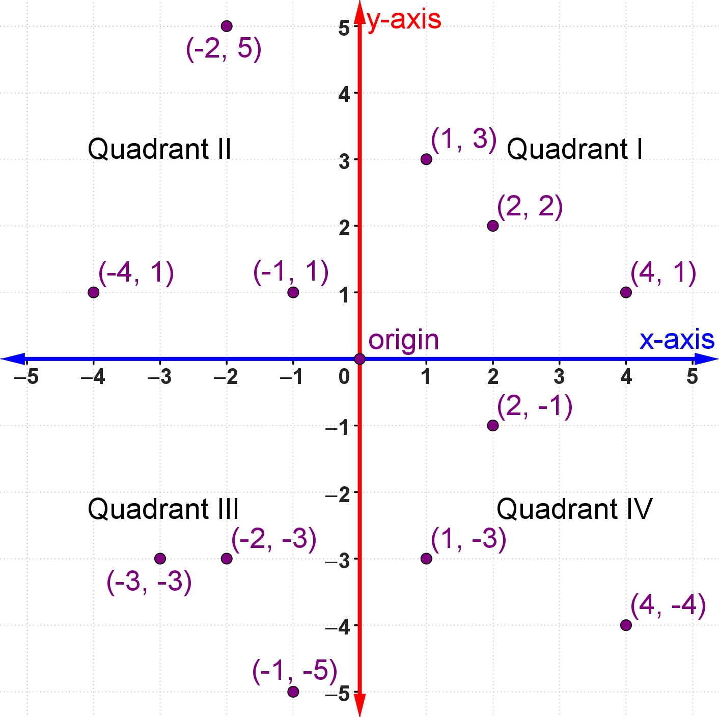
The horizontal axis in the coordinate plane is called the [latex] x [/latex]-axis. The vertical axis is called the [latex] y [/latex]-axis. The point at which the two axes intersect is called the origin. The origin is at [latex]0[/latex] on the [latex] x [/latex]–axis and [latex]0[/latex] on the [latex] y [/latex]–axis.

Locations on the coordinate plane are described as ordered pairs. An ordered pair tells you the location of a point by relating the point’s location along the [latex] x [/latex]–axis (the first value of the ordered pair) and along the [latex] y [/latex]-axis (the second value of the ordered pair).

In an ordered pair, such as [latex] (x,y) [/latex], the first value is called the [latex] x [/latex]-coordinate or the input and the second value is the [latex] y [/latex]-coordinate or the output. Note that the [latex] x [/latex]–coordinate is listed before the [latex] y [/latex]–coordinate. Since the origin has an [latex] x [/latex]–coordinate of [latex]0[/latex] and a [latex] y [/latex]–coordinate of [latex]0[/latex], its ordered pair is written as [latex] (0,0) [/latex].

Consider the point below.

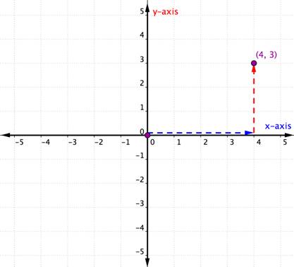
To identify the location of this point, start at the origin [latex] (0,0) [/latex] and move right along the [latex] x [/latex]–axis until you are under the point. Look at the label on the [latex] x [/latex]–axis. The [latex]4[/latex] indicates that, from the origin, you have traveled four units to the right along the [latex] x [/latex]-axis. This is the [latex] x [/latex]–coordinate; the first number in the ordered pair.

From [latex]4[/latex] on the [latex] x [/latex]–axis move up to the point and notice the number with which it aligns on the [latex] y [/latex]–axis. The [latex]3[/latex] indicates that, after leaving the [latex] x [/latex]-axis, you traveled [latex]3[/latex] units up in the vertical direction, the direction of the [latex] y [/latex]-axis. This number is the [latex] y [/latex]–coordinate, the second number in the ordered pair. With an [latex] x [/latex]–coordinate of [latex]4[/latex] and a [latex] y [/latex]–coordinate of [latex]3[/latex], you have the ordered pair [latex] (4,3) [/latex].

Using a Table of Values to Graph a Linear Equation

A helpful first step in graphing an equation is to make a table of values. This is particularly useful when you do not know the general shape the graph will have. You probably already know that the graph of a linear equation will be a straight line, but let us make a table first to see how it can be helpful.

Make a table of values for [latex]y=3x+2[/latex]. It is a good idea to include negative values, positive values, and zero as inputs. Evaluate the given equation for each input value of [latex] x [/latex].

Now use the ordered pairs to help you draw the graph of the equation.

Using a Table of Values to Graph a Quadratic Equation

Not all graphs are straight lines. Next, let’s explore the shape of the graph of a Quadratic Equation. Let’s use a table of values to graph a basic quadratic equation: [latex] y=x^2 [/latex].
Start by creating a table of values, then plot the ordered pairs.

[latex] x [/latex]	[latex] y=x^2 [/latex]	[latex] (x,y) [/latex]
[latex]\color{green}{−2}[/latex]	[latex]y=(\color{green}{-2})^2=4[/latex]	[latex](-2,4)[/latex]
[latex]\color{green}{−1}[/latex]	[latex]y=(\color{green}{-1})^2=1[/latex]	[latex](-1,1)[/latex]
[latex]\color{green}{0}[/latex]	[latex]y=(\color{green}{0})^2=0[/latex]	[latex](0,0)[/latex]
[latex]\color{green}{1}[/latex]	[latex]y=(\color{green}{1})^2=1[/latex]	[latex](1,1)[/latex]
[latex]\color{green}{2}[/latex]	[latex]y=(\color{green}{2})^2=4[/latex]	[latex](2,4)[/latex]

Plot the points [latex](-2,4), (-1,1), (0,0), (1,1), (2,4)[/latex]

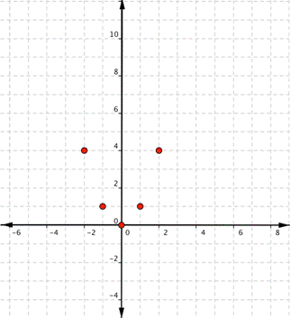
Since the points are not on a line, you cannot use a straight edge. Connect the points as best as you can using a smooth curve (not a series of straight lines). You may want to find and plot additional points (such as the ones in blue here). Placing arrows on the tips of the lines implies that they continue in that direction forever.

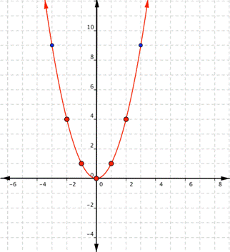
Notice that the shape is similar to the letter U. This is called a parabola. One-half of the parabola is a mirror image of the other half. The lowest point on this graph is called the vertex. The vertical line that goes through the vertex is called the line of reflection. In this case, that line is the [latex] y [/latex]-axis.

Examples

Complete the table of values and graph [latex] y=x^2-3 [/latex].

[latex] x [/latex]	[latex] y=x^2-3 [/latex]	[latex] (x,y) [/latex]
[latex]\color{green}{−2}[/latex]
[latex]\color{green}{−1}[/latex]
[latex]\color{green}{0}[/latex]
[latex]\color{green}{1}[/latex]
[latex]\color{green}{2}[/latex]

Show Solution

[latex] x [/latex]	[latex] y=x^2-3 [/latex]	[latex] (x,y) [/latex]
[latex]\color{green}{−2}[/latex]	[latex]y=(\color{green}{-2})^2-3=1[/latex]	[latex](-2,1)[/latex]
[latex]\color{green}{−1}[/latex]	[latex]y=(\color{green}{-1})^2-3=-2[/latex]	[latex](-1,-2)[/latex]
[latex]\color{green}{0}[/latex]	[latex]y=(\color{green}{0})^2-3=-3[/latex]	[latex](0,-3)[/latex]
[latex]\color{green}{1}[/latex]	[latex]y=(\color{green}{1})^2-3=-2[/latex]	[latex](1,-2)[/latex]
[latex]\color{green}{2}[/latex]	[latex]y=(\color{green}{2})^2-3=1[/latex]	[latex](2,1)[/latex]

Graph the points [latex] (-2,1), (-1,-2), (0,-3), (1,-2), (2,1) [/latex] Then connect the points with a smooth curve.

 

Using a Table of Values to Graph a Square Root Equation

To graph a square root equation [latex] y=\sqrt{x} [/latex] using a table of values, in this example we will only choose [latex] x [/latex]-values that are perfect squares. Doing this makes it much easier to evaluate and plot the points.

[latex] x [/latex]	[latex] y [/latex]	[latex] (x,y) [/latex]
[latex]\color{green}{0}[/latex]	[latex]y=\sqrt{\color{green}{0}}=0[/latex]	[latex](0,0)[/latex]
[latex]\color{green}{1}[/latex]	[latex]y=\sqrt{\color{green}{1}}=1[/latex]	[latex](1,1)[/latex]
[latex]\color{green}{4}[/latex]	[latex]y=\sqrt{\color{green}{4}}=2[/latex]	[latex](4,2)[/latex]
[latex]\color{green}{9}[/latex]	[latex]y=\sqrt{\color{green}{9}}=3[/latex]	[latex](9,3)[/latex]
[latex]\color{green}{16}[/latex]	[latex]y=\sqrt{\color{green}{16}}=4[/latex]	[latex](16,4)[/latex]

Notice that we only used positive or zero values for the inputs to the square root. Recall that [latex] \sqrt{x} [/latex] means to find the number whose square is [latex] x [/latex]. For example, [latex]\sqrt{49}[/latex] means “find the number whose square is [latex]49[/latex].” Since there is no real number that we can square and get a negative, the equation [latex]y=\sqrt{x}[/latex] will be defined for [latex]x>0[/latex].

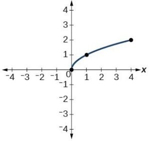
Here’s the graph of [latex] y=\sqrt{x} [/latex].

Example

Complete the table of values and graph [latex] y=\sqrt{(x+4)} [/latex].

[latex] x [/latex]	[latex] y=\sqrt{(x+4)} [/latex]	[latex] (x,y) [/latex]
[latex]\color{green}{-4}[/latex]
[latex]\color{green}{-3}[/latex]
[latex]\color{green}{0}[/latex]
[latex]\color{green}{5}[/latex]
[latex]\color{green}{12}[/latex]

Show Solution

On this example, notice the [latex] x [/latex]-values that we are choosing are not perfect squares like in the explanation above. This time we are choosing [latex] x [/latex]-values that will make the radicand simplify to be a perfect square. An [latex] x [/latex] value of [latex] -3 [/latex] was picked below. Notice when I substitute [latex] -3 [/latex] in place of [latex] x [/latex] in the equation we get [latex] -3+4 [/latex] under the square root. When we simplify that we get [latex] 1 [/latex] and that is a perfect square. Check out the other [latex] x [/latex]-values and notice what happens when you simplify before you take the square root.

[latex] x [/latex]	[latex] y=\sqrt{(x+4)} [/latex]	[latex] (x,y) [/latex]
[latex]\color{green}{-4}[/latex]	[latex] y=\sqrt{(\color{green}{-4}\color{black}{)+4}}=\sqrt{0}=0 [/latex]	[latex](-4,0)[/latex]
[latex]\color{green}{-3}[/latex]	[latex] y=\sqrt{(\color{green}{-3}\color{black}{)+4}}=\sqrt{1}=1 [/latex]	[latex](-3,1)[/latex]
[latex]\color{green}{0}[/latex]	[latex] y=\sqrt{(\color{green}{0}\color{black}{)+4}}=\sqrt{4}=2 [/latex]	[latex](0,2)[/latex]
[latex]\color{green}{5}[/latex]	[latex] y=\sqrt{(\color{green}{5}\color{black}{)+4}}=\sqrt{9}=3 [/latex]	[latex](5,3)[/latex]
[latex]\color{green}{12}[/latex]	[latex] y=\sqrt{(\color{green}{12}\color{black}{)+4}}=\sqrt{16}=4 [/latex]	[latex](12,4)[/latex]

 

Graphs of Common Functions

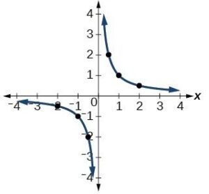
Throughout our course, you’ll use graphs to aid in understanding relationships between input ([latex] x [/latex]) and output ([latex] y [/latex]) variables. Learn to recognize these graphs and their features quickly by name, formula, and graph.

Name	Equation	Graph	Table
Constant	[latex]y=c[/latex], where [latex]c[/latex] is a constant		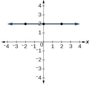[latex] x [/latex] [latex] y [/latex] -2 2 0 2 2 2
Linear	[latex]y=x[/latex]		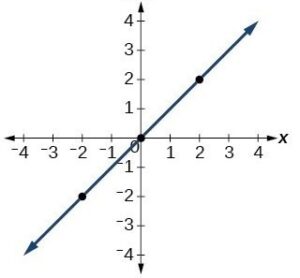[latex] x [/latex] [latex] y [/latex] -2 -2 0 0 2 2
Absolute Value	[latex]y=|x|[/latex]		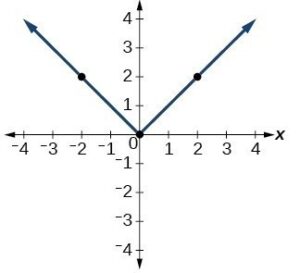[latex] x [/latex] [latex] y [/latex] -2 2 0 0 2 2
Quadratic	[latex]y={x}^{2}[/latex]		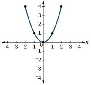[latex] x [/latex] [latex] y [/latex] -2 4 -1 1 0 0 1 1 2 4
Cubic	[latex]y={x}^{3}[/latex]		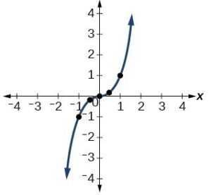[latex] x [/latex] [latex] y [/latex] -1 -1 -0.5 -0.125 0 0 0.5 0.125 1 1
Reciprocal	[latex]y=\frac{1}{x}[/latex] Notice that this equation is not defined for all inputs. We’ll talk more about this in the next section.		[latex] x [/latex] [latex] y [/latex] -2 -0.5 -1 -1 -0.5 -2 0.5 2 1 1 2 0.5
Square root	[latex]y=\sqrt{x}[/latex] Notice that this equation is not defined for all inputs. We’ll talk more about this in the next section.		[latex] x [/latex] [latex] y [/latex] 0 0 1 1 4 2

 

Try It