16.2 Entropy

Learning Objectives

By the end of this section, you will be able to:

Define entropy
Explain the relationship between entropy and the number of microstates
Predict the sign of the entropy change for chemical and physical processes

In 1824, at the age of 28, Nicolas Léonard Sadi Carnot (Figure 1) published the results of an extensive study regarding the efficiency of steam heat engines. In a later review of Carnot’s findings, Rudolf Clausius introduced a new thermodynamic property that relates the spontaneous heat flow accompanying a process to the temperature at which the process takes place. This new property was expressed as the ratio of the reversible heat (q_rev) and the kelvin temperature (T). The term reversible process refers to a process that takes place at such a slow rate that it is always at equilibrium and its direction can be changed (it can be “reversed”) by an infinitesimally small change is some condition. Note that the idea of a reversible process is a formalism required to support the development of various thermodynamic concepts; no real processes are truly reversible, rather they are classified as irreversible.

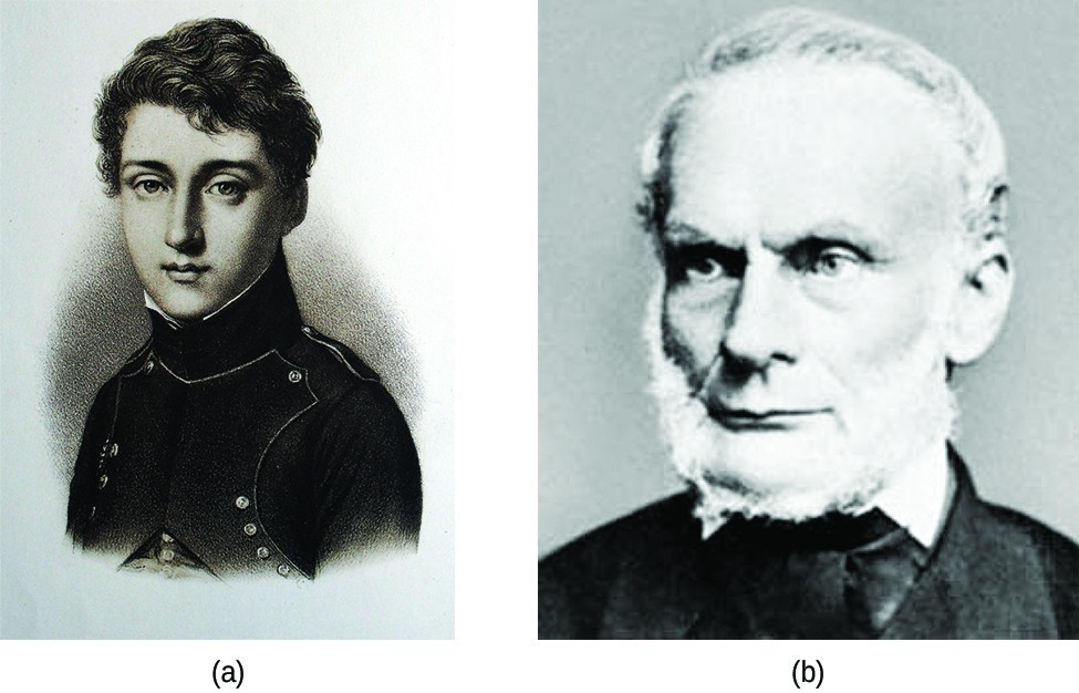
Figure 1. (a) Nicholas Léonard Sadi Carnot’s research into steam-powered machinery and (b) Rudolf Clausius’s later study of those findings led to groundbreaking discoveries about spontaneous heat flow processes.

Similar to other thermodynamic properties, this new quantity is a state function, and so its change depends only upon the initial and final states of a system. In 1865, Clausius named this property entropy (S) and defined its change for any process as the following:

[latex]\Delta S=\frac{{q}_{\text{rev}}}{T}[/latex]

The entropy change for a real, irreversible process is then equal to that for the theoretical reversible process that involves the same initial and final states.

Entropy and Microstates

Following the work of Carnot and Clausius, Ludwig Boltzmann developed a molecular-scale statistical model that related the entropy of a system to the number of microstates possible for the system. A microstate (W) is a specific configuration of the locations and energies of the atoms or molecules that comprise a system like the following:

[latex]S=k\text{ln}W[/latex]

Here k is the Boltzmann constant and has a value of 1.38 [latex]\times[/latex] 10⁻²³ J/K.

As for other state functions, the change in entropy for a process is the difference between its final (S_f) and initial (S_i) values:

[latex]\Delta S={S}_{\text{f}}-{S}_{\text{i}}=k\text{ln}{W}_{\text{f}}-k\text{ln}{W}_{\text{i}}=k\text{ln}\frac{{W}_{\text{f}}}{{W}_{\text{i}}}[/latex]

For processes involving an increase in the number of microstates, W_f > W_i, the entropy of the system increases, ΔS > 0. Conversely, processes that reduce the number of microstates, W_f < W_i, yield a decrease in system entropy, ΔS < 0. This molecular-scale interpretation of entropy provides a link to the probability that a process will occur as illustrated in the next paragraphs.

Consider the general case of a system comprised of N particles distributed among n boxes. The number of microstates possible for such a system is n^N. For example, distributing four particles among two boxes will result in 2⁴ = 16 different microstates as illustrated in Figure 2. Microstates with equivalent particle arrangements (not considering individual particle identities) are grouped together and are called distributions. The probability that a system will exist with its components in a given distribution is proportional to the number of microstates within the distribution. Since entropy increases logarithmically with the number of microstates, the most probable distribution is therefore the one of greatest entropy.

Five rows of diagrams that look like dominoes are shown and labeled a, b, c, d, and e. Row a has one “domino” that has four dots on the left side, red, green, blue and yellow in a clockwise pattern from the top left, and no dots on the right. Row b has four “dominos,” each with three dots on the left and one dot on the right. The first shows a “domino” with green, yellow and blue on the left and red on the right. The second “domino” has yellow, blue and red on the left and green on the right. The third “domino” has red, green and yellow on the left and blue on the right while the fourth has red, green and blue on the left and yellow on the right. Row c has six “dominos”, each with two dots on either side. The first has a red and green on the left and a blue and yellow on the right. The second has a red and blue on the left and a green and yellow on the right while the third has a yellow and red on the left and a green and blue on the right. The fourth has a green and blue on the left and a red and yellow on the right. The fifth has a green and yellow on the left and a red and blue on the right. The sixth has a blue and yellow on the left and a green and red on the right. Row d has four “dominos,” each with one dot on the left and three on the right. The first “domino” has red on the left and a blue, green and yellow on the right. The second has a green on the left and a red, yellow and blue on the right. The third has a blue on the left and a red, green and yellow on the right. The fourth has a yellow on the left and a red, green and blue on the right. Row e has 1 “domino” with no dots on the left and four dots on the right that are red, green, blue and yellow.

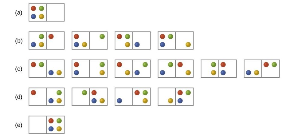
Figure 2. The sixteen microstates associated with placing four particles in two boxes are shown. The microstates are collected into five distributions—(a), (b), (c), (d), and (e)—based on the numbers of particles in each box.

As you add more particles to the system, the number of possible microstates increases exponentially (2^N). A macroscopic (laboratory-sized) system would typically consist of moles of particles (N ~ 10²³), and the corresponding number of microstates would be staggeringly huge. Regardless of the number of particles in the system, however, the distributions in which roughly equal numbers of particles are found in each box are always the most probable configurations.

The previous description of an ideal gas expanding into a vacuum (Figure 3) is a macroscopic example of this particle-in-a-box model. For this system, the most probable distribution is confirmed to be the one in which the matter is most uniformly dispersed or distributed between the two flasks. The spontaneous process whereby the gas contained initially in one flask expands to fill both flasks equally therefore yields an increase in entropy for the system.

A diagram shows two two-sided flasks connected by a right-facing arrow labeled “Spontaneous” and a left-facing arrow labeled “Nonspontaneous.” Each pair of flasks are connected to one another by a tube with a stopcock. In the left pair of flasks, the left flask contains thirty particles evenly dispersed while the right flask contains nothing and the stopcock is closed. The right pair of flasks has an open stopcock and equal numbers of particles in both flasks.

Figure 3. An isolated system consists of an ideal gas in one flask that is connected by a closed valve to a second flask containing a vacuum. Once the valve is opened, the gas spontaneously becomes evenly distributed between the flasks.

A similar approach may be used to describe the spontaneous flow of heat. Consider a system consisting of two objects, each containing two particles, and two units of energy (represented as “*”) in Figure 4. The hot object is comprised of particles A and B and initially contains both energy units. The cold object is comprised of particles C and D, which initially has no energy units. Distribution (a) shows the three microstates possible for the initial state of the system, with both units of energy contained within the hot object. If one of the two energy units is transferred, the result is distribution (b) consisting of four microstates. If both energy units are transferred, the result is distribution (c) consisting of three microstates. And so, we may describe this system by a total of ten microstates. The probability that the heat does not flow when the two objects are brought into contact, that is, that the system remains in distribution (a), is [latex]\frac{3}{10}[/latex]. More likely is the flow of heat to yield one of the other two distribution, the combined probability being [latex]\frac{7}{10}[/latex]. The most likely result is the flow of heat to yield the uniform dispersal of energy represented by distribution (b), the probability of this configuration being [latex]\frac{4}{10}[/latex]. As for the previous example of matter dispersal, extrapolating this treatment to macroscopic collections of particles dramatically increases the probability of the uniform distribution relative to the other distributions. This supports the common observation that placing hot and cold objects in contact results in spontaneous heat flow that ultimately equalizes the objects’ temperatures. And, again, this spontaneous process is also characterized by an increase in system entropy.

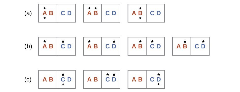
Three rows labeled a, b, and c are shown and each contains rectangles with two sides where the left side is labeled, “A,” and “B,” and the right is labeled, “C,” and “D.” Row a has three rectangles where the first has a dot above and below the letter A, the second has a dot above the A and B, and the third which has a dot above and below the letter B. Row b has four rectangles; the first has a dot above A and C, the second has a dot above A and D, the third has a dot above B and C and the fourth has a dot above B and D. Row c has three rectangles; the first has a dot above and below the letter C, the second has a dot above C and D and the third has a dot above and below the letter D.

Figure 4. This shows a microstate model describing the flow of heat from a hot object to a cold object. (a) Before the heat flow occurs, the object comprised of particles A and B contains both units of energy and as represented by a distribution of three microstates. (b) If the heat flow results in an even dispersal of energy (one energy unit transferred), a distribution of four microstates results. (c) If both energy units are transferred, the resulting distribution has three microstates.

Example 1: Determination of ΔS

Consider the system shown here. What is the change in entropy for a process that converts the system from distribution (a) to (c)?

Show Answer

Check Your Learning

Consider the system shown in Figure 4. What is the change in entropy for the process where all the energy is transferred from the hot object (AB) to the cold object (CD)?

Show Answer

Predicting the Sign of ΔS

The relationships between entropy, microstates, and matter/energy dispersal described previously allow us to make generalizations regarding the relative entropies of substances and to predict the sign of entropy changes for chemical and physical processes. Consider the phase changes illustrated in Figure 5. In the solid phase, the atoms or molecules are restricted to nearly fixed positions with respect to each other and are capable of only modest oscillations about these positions. With essentially fixed locations for the system’s component particles, the number of microstates is relatively small. In the liquid phase, the atoms or molecules are free to move over and around each other, though they remain in relatively close proximity to one another. This increased freedom of motion results in a greater variation in possible particle locations, so the number of microstates is correspondingly greater than for the solid. As a result, S_liquid > S_solid and the process of converting a substance from solid to liquid (melting) is characterized by an increase in entropy, ΔS > 0. By the same logic, the reciprocal process (freezing) exhibits a decrease in entropy, ΔS < 0.

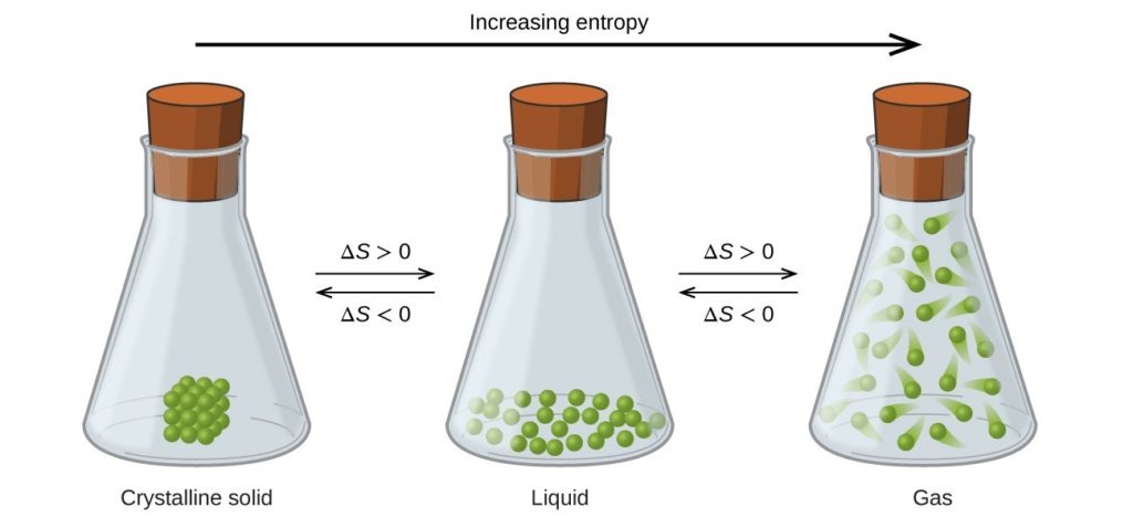
Three stoppered flasks are shown with right and left-facing arrows in between each; the first is labeled above as, “delta S greater than 0,” and below as, “delta S less than 0,” while the second is labeled above as, “delta S greater than 0,” and below as, “delta S less than 0.” A long, right-facing arrow is drawn above all the flasks and labeled, “Increasing entropy.” The left flask contains twenty-seven particles arranged in a cube in the bottom of the flask and is labeled, “Crystalline solid,” below. The middle flask contains twenty-seven particles dispersed randomly in the bottom of the flask and is labeled, “Liquid,” below. The right flask contains twenty-seven particles dispersed inside of the flask and moving rapidly and is labeled, “Gas,” below.

Figure 5. The entropy of a substance increases (ΔS > 0) as it transforms from a relatively ordered solid, to a less-ordered liquid, and then to a still less-ordered gas. The entropy decreases (ΔS < 0) as the substance transforms from a gas to a liquid and then to a solid.

Now consider the vapor or gas phase. The atoms or molecules occupy a much greater volume than in the liquid phase; therefore each atom or molecule can be found in many more locations than in the liquid (or solid) phase. Consequently, for any substance, S_gas > S_liquid > S_solid, and the processes of vaporization and sublimation likewise involve increases in entropy, ΔS > 0. Likewise, the reciprocal phase transitions, condensation and deposition, involve decreases in entropy, ΔS < 0.

According to kinetic-molecular theory, the temperature of a substance is proportional to the average kinetic energy of its particles. Raising the temperature of a substance will result in more extensive vibrations of the particles in solids and more rapid translations of the particles in liquids and gases. At higher temperatures, the distribution of kinetic energies among the atoms or molecules of the substance is also broader (more dispersed) than at lower temperatures. Thus, the entropy for any substance increases with temperature (Figure 6).

Two graphs are shown. The y-axis of the left graph is labeled, “Fraction of molecules,” while the x-axis is labeled, “Velocity, v ( m / s ),” and has values of 0 through 1,500 along the axis with increments of 500. Four lines are plotted on this graph. The first, labeled, “100 K,” peaks around 200 m / s while the second, labeled, “200 K,” peaks near 300 m / s and is slightly lower on the y-axis than the first. The third line, labeled, “500 K,” peaks around 550 m / s and is lower than the first two on the y-axis. The fourth line, labeled, “1000 K,” peaks around 750 m / s and is the lowest of the four on the y-axis. Each line get increasingly broad. The second graph has a y-axis labeled, “Entropy, S,” with an upward-facing arrow and an x-axis labeled, “Temperature ( K ),” and a right-facing arrow. The graph has three equally spaced columns in the background, labeled, “Solid,” “Liquid,” and, “Gas,” from left to right. A line extends slightly upward through the first column in a slight upward direction, then goes straight up in the transition between the first two columns. In then progresses in a slight upward direction through the second column, then goes up dramatically between the second and third columns, then continues in a slight upward direction once more. The first vertical region of this line is labeled, “Melting,” and the second is labeled, “Boiling.”

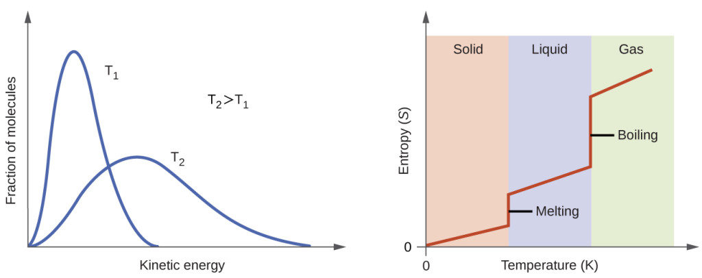
Figure 6. Entropy increases as the temperature of a substance is raised, which corresponds to the greater spread of kinetic energies. When a substance melts or vaporizes, it experiences a significant increase in entropy.

Try this interactive simulation of the dependence of particle location and freedom of motion on physical state and temperature.

The entropy of a substance is influenced by structure of the particles (atoms or molecules) that comprise the substance. With regard to atomic substances, heavier atoms possess greater entropy at a given temperature than lighter atoms, which is a consequence of the relation between a particle’s mass and the spacing of quantized translational energy levels (which is a topic beyond the scope of our treatment). For molecules, greater numbers of atoms (regardless of their masses) increase the ways in which the molecules can vibrate and thus the number of possible microstates and the system entropy.

Finally, variations in the types of particles affects the entropy of a system. Compared to a pure substance, in which all particles are identical, the entropy of a mixture of two or more different particle types is greater. This is because of the additional orientations and interactions that are possible in a system comprised of nonidentical components. For example, when a solid dissolves in a liquid, the particles of the solid experience both a greater freedom of motion and additional interactions with the solvent particles. This corresponds to a more uniform dispersal of matter and energy and a greater number of microstates. The process of dissolution therefore involves an increase in entropy, ΔS > 0.

Considering the various factors that affect entropy allows us to make informed predictions of the sign of ΔS for various chemical and physical processes as illustrated in Example 2.

Example 2: Predicting the Sign of ∆S

Predict the sign of the entropy change for the following processes. Indicate the reason for each of your predictions.

One mole liquid water at room temperature [latex]\longrightarrow[/latex] one mole liquid water at 50 °C
[latex]{\text{Ag}}^{\text{+}}\left(aq\right)+{\text{Cl}}^{-}\left(aq\right)\longrightarrow \text{AgCl}\left(s\right)[/latex]
[latex]{\text{C}}_{6}{\text{H}}_{6}\left(l\right)+\frac{15}{2}{\text{O}}_{2}\left(g\right)\longrightarrow 6{\text{CO}}_{2}\left(g\right)+3{\text{H}}_{2}\text{O}\left(l\right)[/latex]
[latex]{\text{NH}}_{3}\left(s\right)\longrightarrow {\text{NH}}_{\text{3}}\left(l\right)[/latex]

Show Answer

Check Your Learning

Predict the sign of the enthalpy change for the following processes. Give a reason for your prediction.

[latex]{\text{NaNO}}_{3}\left(s\right)\longrightarrow {\text{Na}}^{\text{+}}\left(aq\right)+{\text{NO}}_{3}{}^{-}\left(aq\right)[/latex]
the freezing of liquid water
[latex]{\text{CO}}_{2}\left(s\right)\longrightarrow {\text{CO}}_{2}\left(g\right)[/latex]
[latex]\text{CaCO}\left(s\right)\longrightarrow \text{CaO}\left(s\right)+{\text{CO}}_{2}\left(g\right)[/latex]

Show Answer

Key Concepts and Summary

Entropy (S) is a state function that can be related to the number of microstates for a system (the number of ways the system can be arranged) and to the ratio of reversible heat to kelvin temperature. It may be interpreted as a measure of the dispersal or distribution of matter and/or energy in a system, and it is often described as representing the “disorder” of the system.

For a given substance, S_solid < S_liquid < S_gas in a given physical state at a given temperature, entropy is typically greater for heavier atoms or more complex molecules. Entropy increases when a system is heated and when solutions form. Using these guidelines, the sign of entropy changes for some chemical reactions may be reliably predicted.

Key Equations

[latex]\Delta S=\frac{{q}_{\text{rev}}}{T}[/latex]
S = k ln W
[latex]\Delta S=k\text{ln}\frac{{W}_{\text{f}}}{{W}_{\text{i}}}[/latex]

Exercises

In Figure 2 all possible distributions and microstates are shown for four different particles shared between two boxes. Determine the entropy change, ΔS, if the particles are initially evenly distributed between the two boxes, but upon redistribution all end up in Box (b).
In Figure 2 all of the possible distributions and microstates are shown for four different particles shared between two boxes. Determine the entropy change, ΔS, for the system when it is converted from distribution (b) to distribution (d).
How does the process described in the previous item relate to the system shown in Figure 3?
Consider a system similar to the one in Figure 2, except that it contains six particles instead of four. What is the probability of having all the particles in only one of the two boxes in the case? Compare this with the similar probability for the system of four particles that we have derived to be equal to [latex]\frac{1}{8}[/latex]. What does this comparison tell us about even larger systems?
Consider the system shown in Figure 4. What is the change in entropy for the process where the energy is initially associated only with particle A, but in the final state the energy is distributed between two different particles?
Consider the system shown in Figure 4. What is the change in entropy for the process where the energy is initially associated with particles A and B, and the energy is distributed between two particles in different boxes (one in A-B, the other in C-D)?
Arrange the following sets of systems in order of increasing entropy. Assume one mole of each substance and the same temperature for each member of a set.
1. H₂(g), HBrO₄(g), HBr(g)
2. H₂O(l), H₂O(g), H₂O(s)
3. He(g), Cl₂(g), P₄(g)
At room temperature, the entropy of the halogens increases from I₂ to Br₂ to Cl₂. Explain.
Consider two processes: sublimation of I₂(s) and melting of I₂(s) (Note: the latter process can occur at the same temperature but somewhat higher pressure).
[latex]{\text{I}}_{2}\left(s\right)\longrightarrow {\text{I}}_{2}\left(g\right)[/latex]
[latex]{\text{I}}_{2}\left(s\right)\longrightarrow {\text{I}}_{2}\left(l\right)[/latex]
Is ΔS positive or negative in these processes? In which of the processes will the magnitude of the entropy change be greater?
Indicate which substance in the given pairs has the higher entropy value. Explain your choices.
1. C₂H₅OH(l) or C₃H₇OH(l)
2. C₂H₅OH(l) or C₂H₅OH(g)
3. 2H(g) or H(g)
Predict the sign of the entropy change for the following processes.
1. An ice cube is warmed to near its melting point.
2. Exhaled breath forms fog on a cold morning.
3. Snow melts.
Predict the sign of the enthalpy change for the following processes. Give a reason for your prediction.
1. [latex]{\text{Pb}}^{2+}\left(aq\right)+{\text{S}}^{2-}\left(aq\right)\longrightarrow \text{PbS}\left(s\right)[/latex]
2. [latex]2\text{Fe}\left(s\right)+3{\text{O}}_{2}\left(g\right)\longrightarrow {\text{Fe}}_{2}{\text{O}}_{3}\left(s\right)[/latex]
3. [latex]2{\text{C}}_{6}{\text{H}}_{14}\left(l\right)+19{\text{O}}_{2}\left(g\right)\longrightarrow 14{\text{H}}_{2}\text{O}\left(g\right)+12{\text{CO}}_{2}\left(g\right)[/latex]
Write the balanced chemical equation for the combustion of methane, CH₄(g), to give carbon dioxide and water vapor. Explain why it is difficult to predict whether ΔS is positive or negative for this chemical reaction.
Write the balanced chemical equation for the combustion of benzene, C₆H₆(l), to give carbon dioxide and water vapor. Would you expect ΔS to be positive or negative in this process?

Show Selected Answers

2. There are four initial microstates and four final microstates. [latex]\Delta S=k\text{ln}\frac{{W}_{\text{f}}}{{W}_{\text{i}}}=1.38\times {\text{10}}^{-23}\text{J/K}\times \text{ln}\frac{4}{4}=0[/latex]

4. A system of N particles will have 2N microstates, since each of the particles can be in one of the two states (on the left or on the right), and its probability to be in one of them is independent of positions of the other particles. Therefore, there are 2⁶ = 64 possible microstates for six particles. Only two of them correspond to all the particles being in one box (one for the right box and one for the left box). Thus, the probability for all the particles to be on one side is [latex]\frac{2}{64}=\frac{1}{32}[/latex]. This probability is noticeably lower than the [latex]\frac{1}{8}[/latex] result for the four-particle system. The conclusion we can make is that the probability for all the particles to stay in only one part of the system will decrease rapidly as the number of particles increases, and, for instance, the probability for all molecules of gas to gather in only one side of a room at room temperature and pressure is negligible since the number of gas molecules in the room is very large.

6. There is only one initial state. For the final state, the energy can be contained in pairs A-C, A-D, B-C, or B-D. Thus, there are four final possible states [latex]\Delta S=k\text{ln}\left(\frac{{W}_{\text{f}}}{{W}_{\text{i}}}\right)=1.38\times {10}^{-23}\text{J/K}\times \text{ln}\left(\frac{4}{1}\right)=1.91\times {10}^{-23}\text{J/K}[/latex]

8. The masses of these molecules would suggest the opposite trend in their entropies. The observed trend is a result of the more significant variation of entropy with a physical state. At room temperature, I₂ is a solid, Br₂ is a liquid, and Cl₂ is a gas.

10. The correct answers are as follows:

C₃H₇OH(l) as it is a larger molecule (more complex and more massive), and so more microstates describing its motions are available at any given temperature.
C₂H₅OH(g) as it is in the gaseous state.
2H(g), since entropy is an extensive property, and so two H atoms (or two moles of H atoms) possess twice as much entropy as one atom (or one mole of atoms).

12. The predicted signs are as follows:

Negative. The relatively ordered solid precipitating decreases the number of mobile ions in solution.
Negative. There is a net loss of three moles of gas from reactants to products.
Positive. There is a net increase of seven moles of gas from reactants to products.

14. [latex]\text{C}_{6}\text{H}_{6}\left(l\right)+7.5\text{O}_{2}\left(g\right)\longrightarrow3\text{H}_{2}\text{O}\left(g\right)+6\text{CO}_{2}\left(g\right)[/latex]
There are 7.5 moles of gas initially, and 3 + 6 = 9 moles of gas in the end. Therefore, it is likely that the entropy increases as a result of this reaction, and ΔS is positive.

Glossary

entropy (S): state function that is a measure of the matter and/or energy dispersal within a system, determined by the number of system microstates often described as a measure of the disorder of the system

microstate (W): possible configuration or arrangement of matter and energy within a system

reversible process: process that takes place so slowly as to be capable of reversing direction in response to an infinitesimally small change in conditions; hypothetical construct that can only be approximated by real processes removed

Chapter 16: Thermodynamics

Learning Objectives

Entropy and Microstates

Example 1: Determination of ΔS

Check Your Learning

Predicting the Sign of ΔS

Example 2: Predicting the Sign of ∆S

Check Your Learning

Key Concepts and Summary

Key Equations

Exercises

Glossary

Candela Citations