Learning Objectives
- Explain what we mean by object-oriented programming.
- Apply the fundamental concepts of computer graphics in a computer program.
- Create objects in programs and use methods to perform graphical computations.
- Write simple interactive graphics programs using objects available in the graphics module.
- Read and write programs that define functions and use function calls and parameter passing in Python.
Object Oriented Programming
Python is a multi-paradigm programming language, meaning it supports different programming approaches. In general, there are four main programming paradigms, logical, imperative, functional and object-oriented, with object-oriented being the most recent. Object-Oriented Programming’s (OOP) approach to solving computational problems is by creating objects, which may contain data, in the form of fields (attributes), and code, in the form of procedures (methods).
Object-Oriented Programming allows us to define, create and manipulate objects. Another feature of objects is that an object’s procedures can access and often modify the data fields of the object with which they are associated. In OOP, computer programs are designed by making them out of objects that interact with one another.
There is significant diversity of OOP languages, but the most popular ones, including Python, are class-based, meaning that objects are instances of classes, which determine their data type.
It can be shown that anything solvable using one of these paradigms can be solved using the others; however, certain types of computational problems lend themselves more naturally to specific paradigms.
Using Objects
We have been using string objects—instances of class str—for some time. Objects bundle data and functions together, and the data that comprise a string consist of the sequence of characters that make up the string. Strings are objects, and strings “know how” to produce an uppercase version of themselves. For example, examine the following Python statements:
str = 'Hello!'
|
Here upper is a method associated with strings. This means upper is a function that is bound to the string before the dot. This function is bound both logically, and as we see in the new notation, also syntactically. One way to think about it is that each type of data knows operations (methods) that can be applied to it. The expression str.upper() calls the method upper that is bound to the string str and returns a new uppercase string result based on the variable str.
Strings are immutable, so no string method can change the original string, it can only return a new string. Confirm this by entering each line individually in the Python IDLE Shell to see the original str is unchanged:
>>> str = "hello"
>>>
>>> >>>
>>>
>>> |
We are using the new object syntax:
object.method( )
meaning that the method associated with the object’s type is applied to the object. This is just a special syntax for a function call with an object.
Another string method is lower, analogous to upper, but producing a lowercase result.
Many methods also take additional parameters between the parentheses, using the more general syntax:
object.method(parameters)
One such method is count():
Syntax for count: str.count(sub)
The method count() returns the number of repetitions of a string sub that appear as substrings inside the string str. Try this in the Python Shell:
>>> tale = 'This is the best of times. '
>>>
>>> 3 >>> 2 >>> 0 >>> 6 >>> |
There is a blank space between the words in the string 'This is the best of times. ' above and an extra space at the end of the string. Blanks are characters like any other, except we can’t see them.
Just as the parameter can be replaced by a literal value or any expression, the object to which a method is bound with the dot may also be given by a literal value, or a variable name, or any expression that evaluates to the right kind of object in its place. This is true for any method call.
Technically the dot between the object and the method name is an operator, and operators have different levels of precedence. It is important to realize that this dot operator has the highest possible precedence. Read and see the difference parentheses make in the expressions (try this too!):
>>> 'hello ' + 'there'.upper()
>>>
|
Python lets you see all the methods that are bound to an object (and any object of its type) with the built-in function dir. To see all string methods, supply the dir function with any string. For example, try in the Python IDLE Shell:
dir('')
Many of the names in the list start and end with two underscores, like __add__. These are all associated with methods and pieces of data used internally by the Python interpreter. You can ignore them for now. The remaining entries in the list are all user-level methods for strings. You should see lower and upper among them. Some of the methods are much more commonly used than others.

Figure 22: List of String Methods
Object notation:
object.method(parameters)
has been illustrated so far with just the object type str, but it applies to all types including integers and floating-point numbers.
In summary (Figure 23), objects are simply variables that are some defined data type (e.g. the variable “age” is an “integer” type). Objects have data associated with them (e.g. the variable “age” is assigned the value of 15 in the Python statement age = 15). To perform an operation (or procedure) on an object, we send the object a message. The set of messages an object responds to are called the methods of the object (e.g. the Python statement print(age))
- Methods are like functions that live inside the object.
- Methods are invoked using dot-notation:
<object>.<method-name>(<param1>, <param2>, …)

Figure 23: “Object Oriented Programming Python Code” by Miles J. Pool is licensed under CC-BY 4.0
Simple Graphics Programming
Graphics make programming more fun for many people. To fully introduce graphics would involve many ideas that would be a distraction now. This section introduces a simplified object oriented graphics library developed by John Zelle for use with his Python Programming book. The graphics library was designed to make it easy for novice programmers to experiment with computer graphics in an object oriented fashion.
There are two kinds of objects in the library. The GraphWin class implements a window where drawing can be done, and various graphics objects (like circles and squares) are provided that can be drawn into a GraphWin.
In order to use this module and build graphical programs you will need a copy of graphics.py. You can download this from http://mcsp.wartburg.edu/zelle/python/graphics.py . You will want to place this file (graphics.py) in the same folder you use for all your Python programs (the files with the .py extension).
graphics.py code, so you do not need to understand the inner workings! It uses all sorts of features of Python that are way beyond the scope of this book. There is no particular need to open graphics.py in the Python IDLE editor.Once the module is downloaded (therefore ‘installed’), we can import it just like a library that is built into Python like math:
import graphics
If typing this line in the Python IDLE Shell gives you no output, then you have installed the graphics module correctly! If there is an error message, then Python could not find the graphics.py file.
We will begin with a simple example program, graphIntroSteps.py[1], which you can download from here:
www.pas.rochester.edu/~rsarkis/csc161/_static/idle/examples/graphIntroSteps.py
Copy this .py file into the same folder that you copied the graphics.py file to and run it. Each time you press return, look at the screen and read the explanation for the next line(s).
Look around on your screen, and possibly underneath other windows: There should be a new window labeled “Graphics Window”, created by the second line. Bring it to the top, and preferably drag it around to make it visible beside your Shell window. A GraphWin is a type of object from Zelle’s graphics package that automatically displays a window when it is created. The assignment statement remembers the window object as win for future reference. (This will be our standard name for our graphics window object.) A small window, 200 by 200 pixels is created. A pixel is the smallest little square that can be displayed on your screen. Modern screens usually have more than 1000 pixels across the whole screen. A pixel is the basic unit of programmable color on a computer display or in a computer image.
The example program graphIntro.py starts with the same graphics code as graphIntoSteps.py, but without the need for pressing returns.
Added to this program is the ability to print a string value of graphics objects for debugging purposes. If some graphics object isn’t visible because it is underneath something else or off the screen, temporarily adding this sort of output will help you debug your code. Let us examine each line of code in this graphics program.
|
Python Statement |
Explanation |
|
|
Zelle’s graphics are not a part of the standard Python distribution. For the Python interpreter to find Zelle’s module, it must be imported. |
|
|
A GraphWin is a type of object that automatically displays a window when it is created. A small window, 200 by 200 pixels is created. |
|
|
This creates a Point object and assigns it the name pt. A Point object, like each of the graphical objects that can be drawn on a GraphWin, has a method draw. |
|
|
Now you should see the Point if you look hard in the Graphics Window – it shows as a single, small, black pixel. |
|
|
This creates a Circle object with center at the previously defined pt and with radius 25. |
|
|
Now you should see the Circle in the Graphics Window. |
|
|
Uses method setOutline to color the object’s border. |
|
|
Uses method setFill to color the inside of the object. |
|
|
A Line object is constructed with two Points as parameters. In this case we use the previously named Point, pt, and specify another Point directly. |
|
|
Technically the Line object is a segment between the the two points. You should now see the line in the Graphics Window. |
|
|
A rectangle is also specified by two points. The points must be diagonally opposite corners. |
|
|
The drawn Rectangle object is restricted to have horizontal and vertical sides. |
|
|
The parameters to the move method are the amount to shift the x and y coordinates of the object. The line will visibly move in the Graphics Window. |
|
|
These three lines are used for debugging purposes. The coordinates for each object will be displayed in the Shell. |
|
|
This statement displays instructions (in the Shell) for the user. |
|
|
The Graphics Window is closed (it disappears). |
Table 4: Python graphIntro.py Code Explained
Figure 24 shows the Graphics Window created by graphIntroSteps.py with the various graphics objects displayed in it. Next, in Figure 25, is the output that is displayed in the Python IDLE Shell. Once the user presses the Enter key (‘return’) the Graphics Window disappears.

Figure 24: Example Graphics Window

Figure 25: Python Idle Shell Output
Graphics Windows: Coordinate Systems
Graphics windows have a Cartesian (x,y) coordinate system. The dimensions are initially measured in pixels. The first coordinate is the horizontal coordinate, measured from left to right, so in the default 200×200 window, 100 is about half way across the 200 pixel wide window. The second coordinate, for the vertical direction, increases going down from the top of the window by default, not up as you are likely to expect from geometry or algebra class. The coordinate 100 out of the total 200 vertically should be about 1/2 of the way down from the top. See figure 26.

Figure 26: Default Graphics Coordinate System
Much of the graphics programming we will attempt will be based on designing simple GUIs (Graphical User Interfaces) based on some of the programs we have already written. Graphical user interfaces (GUIs) are human-computer interfaces allowing users to interact with an app. Rarely will you find a computer application today that doesn’t have some sort of graphical interface to use it. A graphical interface consists of a window which is populated by “widgets”, the basic building blocks of a GUI. Widgets are the pieces of a GUI that make it usable, e.g. buttons, icons, menu items, on-screen text boxes for typing in information, etc. Basically, anything the user can see in the window is a widget.
Placing and drawing objects in a window defined by pixels (creating images on the pixel level) can get very tedious. The graphics.py module provides us with the ability to set the coordinate system of the window using the setCoords method, which we will see in the following section.
GraphWin Objects
A GraphWin object represents a window on the screen where graphical images may be drawn[2]. A program may define any number of GraphWins. A GraphWin understands the following methods. Recall
GraphWin(title, width, height)
Constructs a new graphics window for drawing on the screen.
The parameters are optional; the default title is “Graphics Window” and the default size is 200 x 200 pixels.
Example: win = GraphWin("My App", 500, 180)
The following figure shows the resulting graphics window which is 500 pixels wide and 180 pixels high with a title of “My App”.

Figure 27: Default Graphics Window
setBackground(color) Sets the window background to the given color. The default background color depends on your system. See Section Generating Colors for information on specifying colors.
Example: win.setBackground("white")
close() Closes the on-screen window.
Example: win.close()
getMouse() Pauses for the user to click a mouse in the window and returns where the mouse was clicked as a Point object.
Example: clickPoint = win.getMouse()
setCoords(x1, y1, x2, y2) Sets the coordinate system of the window. The lower-left corner is (x1; y1) and the upper-right corner is (x2; y2).
Example: win.setCoords(0, 0, 4.0, 4.0)
Example Program Using Coordinate Transformation
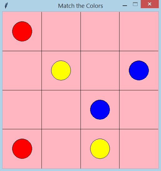
Figure 28: Match the Colors Game
Suppose we wanted to create a simple game app where the user needed to match a pair of tiles with the goal of eventually pair-matching all the tiles in the grid. For example, the user might need to pair matching colored circles as seen here in Figure 28 by clicking on an empty pink square
Drawing the objects of this GUI is certainly easier using coordinate transformation; e.g. defining the coordinate system of our GUI window to go from (0,0) in the lower left corner to (4,4) in the upper right corner).
Examine the code below (matchColorsGame.py).
from graphics import *
win = GraphWin("Match the Colors", 500, 500) #create a 500x500 window
# set coordinates to go from (0,0) in the lower left corner to
# (4,4) in the upper right.
win.setCoords(0.0, 0.0, 4.0, 4.0) ←
win.setBackground("LightPink")
# Draw the vertical lines
Line(Point(1,0), Point(1,4)).draw(win)
Line(Point(2,0), Point(2,4)).draw(win)
Line(Point(3,0), Point(3,4)).draw(win)
# Draw the horizontal lines
Line(Point(0,1), Point(4,1)).draw(win)
Line(Point(0,2), Point(4,2)).draw(win)
Line(Point(0,3), Point(4,3)).draw(win)
# Draw cirlcles in boxes
circle1 = Circle(Point(.5,.5), .25)
circle1.setFill('Red')
circle1.draw(win)
circle2 = Circle(Point(2.5,1.5), .25)
circle2.setFill('Blue')
circle2.draw(win)
circle3 = Circle(Point(1.5,2.5), .25)
circle3.setFill('Yellow')
circle3.draw(win)
circle4 = Circle(Point(3.5,2.5), .25)
circle4.setFill('Blue')
circle4.draw(win)
circle5 = Circle(Point(.5,3.5), .25)
circle5.setFill('Red')
circle5.draw(win)
circle6 = Circle(Point(2.5,.5), .25)
circle6.setFill('Yellow')
circle6.draw(win)
# wait for click and then quit
win.getMouse()
win.close()
Our program still defines the size of the window in pixels (the shaded area in the figure below), but the placement of objects in the window uses the coordinates defined using the win.setCoords method. See Figure 29.

Figure 29: Transformed Graphics Coordinate System
Graphics Objects
The Graphics library provides the following classes of drawable objects: Point, Line, Circle, Oval, Rectangle, Polygon, and Text. All objects are initially created unfilled with a black outline. All graphics objects support the following generic set of methods:
setFill(color) Sets the interior of the object to the given color.
Example: someObject.setFill("red")
setOutline(color) Sets the outline of the object to the given color.
Example: someObject.setOutline("yellow")
setWidth(pixels) Sets the width of the outline of the object to the desired number of pixels. (Does not work for Point.)
Example: someObject.setWidth(3)
draw(aGraphWin) Draws the object into the given GraphWin and returns the drawn object.
Example: someObject.draw(someGraphWin)
move(dx,dy) Moves the object dx units in the x direction and dy units in the y direction. If the object is currently drawn, the image is adjusted to the new position.
Example: someObject.move(10, 15.5)
Point Methods
Point(x,y) Constructs a point having the given coordinates.
Example: aPoint = Point(3.5, 8)
getX() Returns the x coordinate of a point.
Example: xValue = aPoint.getX()
getY() Returns the y coordinate of a point.
Example: yValue = aPoint.getY()
Line Methods
Line(point1, point2) Constructs a line segment from point1 to point2.
Example: aLine = Line(Point(1,3), Point(7,4))
setArrow(endString) Sets the arrowhead status of a line. Arrows may be drawn at either the first point, the last point, or both. Possible values of endString are "first", "last", "both", and "none". The default setting is "none".
Example: aLine.setArrow("both")
getCenter() Returns a clone of the midpoint of the line segment.
Example: midPoint = aLine.getCenter()
getP1(), getP2() Returns a clone of the corresponding endpoint of the segment.
Example: startPoint = aLine.getP1()
Circle Methods
Circle(centerPoint, radius) Constructs a circle with the given center point and radius.
Example: aCircle = Circle(Point(3,4), 10.5)
getCenter() Returns a clone of the center point of the circle.
Example: centerPoint = aCircle.getCenter()
getRadius() Returns the radius of the circle.
Example: radius = aCircle.getRadius()
getP1(), getP2() Returns a clone of the corresponding corner of the circle’s bounding box. These are opposite corner points of a square that circumscribes the circle.
Example: cornerPoint = aCircle.getP1()
Rectangle Methods
Rectangle(point1, point2) Constructs a rectangle having opposite corners at point1 and point2.
Example: aRectangle = Rectangle(Point(1,3), Point(4,7))
getCenter() Returns a clone of the center point of the rectangle.
Example: centerPoint = aRectangle.getCenter()
getP1(), getP2() Returns a clone of the corresponding point used to construct the rectangle.
Example: cornerPoint = aRectangle.getP1()
Oval Methods
Oval(point1, point2) Constructs an oval in the bounding box determined by point1 and point2.
Example: anOval = Oval(Point(1,2), Point(3,4))
getCenter() Returns a clone of the point at the center of the oval.
Example: centerPoint = anOval.getCenter()
getP1(), getP2() Returns a clone of the corresponding point used to construct the oval.
Example: cornerPoint = anOval.getP1()
Polygon Methods
Polygon(point1, point2, point3, ...) Constructs a polygon with the given points as vertices. Also accepts a single parameter that is a list of the vertices.
Example: aPolygon = Polygon(Point(1,2), Point(3,4), Point(5,6))
Example: aPolygon = Polygon([Point(1,2), Point(3,4), Point(5,6)])
getPoints() Returns a list containing clones of the points used to construct the polygon.
Example: pointList = aPolygon.getPoints()
Text Methods
Text(anchorPoint, textString) Constructs a text object that displays textString centered at anchorPoint. The text is displayed horizontally.[3]
Example: message = Text(Point(3,4), "Hello!")
setText(string) Sets the text of the object to string.
Example: message.setText("Goodbye!")
getText() Returns the current string.
Example: msgString = message.getText()
getAnchor() Returns a clone of the anchor point.
Example: centerPoint = message.getAnchor()
setFace(family) Changes the font face to the given family. Possible values are "helvetica", "courier", "times roman", and "arial".
Example: message.setFace("arial")
setSize(point) Changes the font size to the given point size. Sizes from 5 to 36 points are legal.
Example: message.setSize(18)
setStyle(style) Changes font to the given style. Possible values are: "normal", "bold", "italic", and "bold italic".
Example: message.setStyle("bold")
setTextColor(color) Sets the color of the text to color.
Example: message.setTextColor("pink")
Entry Objects
Objects of type Entry are displayed as text entry boxes that can be edited by the user of the program. Entry objects support the generic graphics methods move(), draw(graphwin), undraw(), setFill(color), and clone(). The Entry specific methods are given below.[4]
Entry(centerPoint, width) Constructs an Entry having the given center point and width. The width is specified in number of characters of text that can be displayed.
Example: inputBox = Entry(Point(3,4), 5)
getAnchor() Returns a clone of the point where the entry box is centered.
Example: centerPoint = inputBox.getAnchor()
getText() Returns the string of text that is currently in the entry box.
Example: inputStr = inputBox.getText()
setText(string) Sets the text in the entry box to the given string.
Example: inputBox.setText("32.0")
setFace(family) Changes the font face to the given family. Possible values are "helvetica", "courier", "times roman", and "arial".
Example: inputBox.setFace("courier")
setSize(point) Changes the font size to the given point size. Sizes from 5 to 36 points are legal.
Example: inputBox.setSize(12)
setStyle(style) Changes font to the given style. Possible values are: "normal", "bold", "italic", and "bold italic".
Example: inputBox.setStyle("italic")
setTextColor(color) Sets the color of the text to color.
Example: inputBox.setTextColor("green")
Displaying Images
The Graphics library also provides minimal support for displaying and manipulating images in a GraphWin. Most platforms will support at least PPM and GIF images. Display is done with an Image object. Images support the generic methods move(dx,dy), draw(graphwin), undraw(), and clone(). Image-specific methods are given below.[5]
Image(anchorPoint, filename) Constructs an image from contents of the given file, centered at the given anchor point. Can also be called with width and height parameters instead of filename. In this case, a blank (transparent) image is created of the given width and height (in pixels).
Example: flowerImage = Image(Point(100,100), "flower.gif")
Example: blankImage = Image(320, 240)
getAnchor() Returns a clone of the point where the image is centered.
Example: centerPoint = flowerImage.getAnchor()
getWidth() Returns the width of the image.
Example: widthInPixels = flowerImage.getWidth()
getHeight() Returns the height of the image.
Example: heightInPixels = flowerImage.getHeight()
getPixel(x, y) Returns a list [red, green, blue] of the RGB values of the pixel at position (x,y). Each value is a number in the range 0-255 indicating the intensity of the corresponding RGB color. These numbers can be turned into a color string using the color_rgb function (see next section).
Note that pixel position is relative to the image itself, not the window where the image may be drawn. The upper-left corner of the image is always pixel (0,0).
The following example, displayImage.py, illustrates code that displays a GIF image in a Graphics window The window’s dimensions are determined by variables created by assigning the image’s width and height with the getWidth() and getHeight() methods. The GIF image is 300 x 300 pixels, so the window is 300 x 300. Point is set to coordinates 150 x and 150 y so the image will be centered.

Figure 30: Display an Image Parrots at Sarasota Jungle Gardens by Karen Blaha is licensed under under CC-BY 2.0
Image colors can be adjusted.
Example: red, green, blue = flowerImage.getPixel(32,18)
setPixel(x, y, color) Sets the pixel at position (x,y) to the given color. Note: This is a slow operation.
Example: flowerImage.setPixel(32, 18, "blue")
save(filename) Saves the image to a file. The type of the resulting file (e.g., GIF or PPM) is determined by the extension on the filename.
Example: flowerImage.save("mypic.ppm")
The following example, colortoGrayscale.py, illustrates code that displays a GIF image in a Graphics window, changes the color to grayscale using the setPixel() method, then saves a grayscale copy of the image.

Figure 31: Convert an Image to Grayscale Parrots at Sarasota Jungle Gardens by Karen Blaha is licensed under under CC-BY 2.0
Generating Colors
Colors are indicated by strings. Most normal colors such as “red”, “purple”, “green”, “cyan”, etc. are available. Many colors come in various shades, such as “red1”, “red2″,”red3”, “red4”, which are increasingly darker shades of red. For a full list, see the table below.[6]
The graphics module also provides a function for mixing your own colors numerically. The function color_rgb(red, green, blue) will return a string representing a color that is a mixture of the intensities of red, green and blue specified. These should be ints in the range 0-255. Thus color_rgb(255, 0, 0) is a bright red, while color_rgb(130, 0, 130) is a medium magenta.
Example: aCircle.setFill(color_rgb(130, 0, 130))
|
‘AliceBlue’ |
‘firebrick’ |
‘MistyRose’ |
|
‘AntiqueWhite’ |
‘ForestGreen’ |
‘navy’ |
|
‘aquamarine’ |
‘gold’ |
‘navy blue’ |
|
‘azure’ |
‘gray’ |
‘OliveDrab’ |
|
‘beige’ |
‘gray1’ |
‘orange’ |
|
‘black’ |
‘gray2’ |
‘OrangeRed’ |
|
‘BlanchedAlmond’ |
‘gray3’ |
‘orchid’ |
|
‘blue’ |
‘gray99’ |
‘PaleGreen’ |
|
‘BlueViolet’ |
‘green’ |
‘PaleTurquoise’ |
|
‘brown’ |
‘GreenYellow’ |
‘PaleTurquoise1’ |
|
‘CadetBlue’ |
‘honeydew’ |
‘PaleVioletRed’ |
|
‘chartreuse’ |
‘HotPink’ |
‘PapayaWhip’ |
|
‘chocolate’ |
‘IndianRed’ |
‘PeachPuff’ |
|
‘coral’ |
‘ivory’ |
‘peru’ |
|
‘CornflowerBlue’ |
‘khaki’ |
‘pink’ |
|
‘cornsilk’ |
‘lavender’ |
‘plum’ |
|
‘cyan’ |
‘LavenderBlush’ |
‘PowderBlue’ |
|
‘cyan1’ |
‘LawnGreen’ |
‘purple’ |
|
‘cyan2’ |
‘LemonChiffon’ |
‘red’ |
|
‘cyan3’ |
‘light grey’ |
‘RoyalBlue’ |
|
‘cyan4’ |
‘light slate gray’ |
‘SaddleBrown’ |
|
‘DarkBlue’ |
‘LightBlue’ |
‘salmon’ |
|
‘DarkCyan’ |
‘LightCoral’ |
‘salmon1’ |
|
‘DarkGoldenrod’ |
‘LightCyan’ |
‘salmon2’ |
|
‘DarkGray’ |
‘LightGoldenrod’ |
‘salmon3’ |
|
‘DarkGreen’ |
‘LightGreen’ |
‘salmon4’ |
|
‘DarkGrey’ |
‘LightPink’ |
‘sandy brown’ |
|
‘DarkKhaki’ |
‘LightSalmon’ |
‘SandyBrown’ |
|
‘DarkMagenta’ |
‘LightSeaGreen’ |
‘SeaGreen’ |
|
‘DarkOliveGreen’ |
‘LightSkyBlue’ |
‘seashell’ |
|
‘DarkOrange’ |
‘LightSlateBlue’ |
‘sienna’ |
|
‘DarkOrchid’ |
‘LightSteelBlue’ |
‘SkyBlue’ |
|
‘DarkRed’ |
‘LightYellow’ |
‘SlateBlue’ |
|
‘DarkSalmon’ |
‘LimeGreen’ |
‘SpringGreen’ |
|
‘DarkSeaGreen’ |
‘maroon’ |
‘SpringGreen1’ |
|
‘DarkSlateBlue’ |
‘MediumAquamarine’ |
‘SteelBlue’ |
|
‘DarkSlateGray’ |
‘MediumOrchid’ |
‘tan’ |
|
‘DarkTurquoise’ |
‘MediumPurple’ |
‘turquoise’ |
|
‘DarkViolet’ |
‘MediumSpringGreen’ |
‘violet’ |
|
‘DeepPink’ |
MediumTurquoise’ |
‘VioletRed’ |
|
‘DeepSkyBlue’ |
‘MediumVioletRed’ |
‘yellow’ |
|
‘DimGray’ |
‘MidnightBlue’ |
‘YellowGreen’ |
Table 5: Graphics Library Color Names
Interactive Graphics
In a GUI environment, users interact with their applications by clicking on buttons, choosing items from menus, and typing information into on-screen text boxes. Event-driven programming draws interface elements (widgets) on the screen and then waits for the user to do something. An event is generated whenever a user moves the mouse, clicks the mouse, or types a key on the keyboard.
One limitation of the graphics.py module is that it is not robust if a graphics window is closed by clicking on the standard operating system close button on the title bar. If you close a graphics window that way, you are likely to get a Python error message. On the other hand, if your program creates a graphics window and then terminates abnormally due to some other error, the graphics window may be left orphaned. In this case the close button on the title bar is important: it is the easiest method to clean up and get rid of the window!
This lack of robustness is tied to the simplification designed into the graphics module. If the programmer wants user input, only one type can be specified at a time (either a mouse click in the graphics window via the getMouse method, or via the input keyboard Entry methods into the Shell window).
In graphIntro.py, a prompt to end the graphics program appeared in the Shell window, requiring you to pay attention to two windows.
input("Press return to end")
win.close()
In matchColorsGame.py,where all the action takes place in the graphics window, the only interaction is to click the mouse to close the graphics window. But as mentioned, clicking the standard operating system close button on the title bar will cause a Python Error. To close the graphics window without an error the user must click inside the window.
# wait for click and then quit
win.getMouse()
win.close()
Mouse Clicks
As we have seen in earlier examples, we can get graphical information from the user via the getMouse method of the GraphWin class. The code win.getMouse() waits for a mouse click. In the following code, the position of the mouse click is not important.
# wait for click and then quit
win.getMouse()
win.close()
When getMouse is invoked on a GraphWin, the program pauses and waits for the user to click the mouse somewhere in the window. The spot where the user clicked is returned as a Point object.
The next example, triangle.py[7], illustrates similar starting and ending code. In addition it explicitly interacts with the user. Rather than the code specifying literal coordinates for all graphical objects, the program remembers the places where the user clicks the mouse (stored in variables), and uses them as the vertices of a triangle.

Figure 32: triangle.py
Let us examine the code in this graphics program.
|
Python Statement |
Explanation |
|
|
The standard starting lines (except for the specific values chosen for the width, height, and title of the window). The background color is a property of the whole graphics window that you can set. |
|
|
A Text object is created. This is the prompt for user action. These lines illustrate most of the ways the appearance of a Text object may be modified, with results like in most word processors. |
|
|
After the prompt, the program looks for a response. The win.getMouse() method (with no parameters), waits for you to click the mouse inside win. Then the Point where the mouse was clicked is returned. In this code three mouse clicks are waited for, remembered in variables p1, p2, and p3, and the points are drawn. |
|
|
Next we see a very versatile type of graphical object, a Polygon, which may have any number of vertices specified in a list as its parameter. We see that the methods setFill and setOutline that we used earlier on a Circle, and the setWidth method we used for a Line, also apply to a Polygon, (and also to other graphics objects). |
|
|
Besides changing the style of a Text object, the text itself may be changed as we see in the first line. The remaining code are standard ending lines. |
Tip: Trying to figure out where to place objects in GraphWin can be time consuming and more than likely you will to need to adjust the positions of objects by trial and error until you get the positions you want. We can also print a descriptive string for each graphical type for debugging our graphics code. It only shows position, not other parts of the state of the object.
>>> pt = Point(30, 50)
>>> print(pt) Point(30, 50)
>>> ln = Line(pt)
Point(100, 150))
>>> print(ln)
Line(Point(30, 50), Point(100, 150))
Handling Textual Input
In the triangle.py example, all of the user input was provided through simple mouse clicks. The graphics module also provides a way for the user to enter text inside a textbox via the keyboard with the Entry type. This capability allows us to create primitive (but fully functional!) graphical user interfaces (GUIs). The Entry object is a partial replacement for the input function.
Let us look at a simple example, greet.py, which is presented below:
# Simple example with Entry objects (textboxes).
# Enter your name, click the mouse, and see greetings.
from graphics import *
win = GraphWin("Greeting", 300, 300)
win.setBackground('LightGreen')
instructions = Text(Point(150,35),
"Enter your name.\nThen click the mouse twice.")
instructions.draw(win) #display instructions
entry1 = Entry(Point(150, 230),10) #define the textbox
entry1.draw (win) #draw the textbox
Text(Point (60, 230),'Name:').draw(win) # label for the textbox
win.getMouse() # To know the user is finished with the text.
name = entry1.getText() #assign the text entered to the variable 'name'
greeting1 = 'Hello, 'name'!'# first greeting
Text(Point(110, 160), greeting1).draw(win)
greeting2 = 'Bonjour, 'name'!'# second greeting
Text(Point(160, 120), greeting2).draw(win)
win.getMouse() # To close the window
win.close()

Figure 33: greeting.py Updated Window

Figure 34: greeting.py Updated Window

Figure 35: greeting.py with Coordinate Transformation
When we run this program the window displays (Figure 33), which allows the user to enter in a name.
The user then enters a name into the textbox in the window and is then instructed to ‘click the mouse. Once the user clicks her mouse the first time, the window is updated to reflect the “greetings” as seen here in the second window (Figure 33). The user is also instructed to click her mouse again, which ends the program and closes the window.
The last two graphics program, triangle.py and greeting.py, placed and drew objects in a window defined by pixels which required needing to adjust the positions of objects by trial and error until we got the positions we wanted. This can become very tedious, very fast.
Let us look at how we can instead use coordinate transformation to more easily place and draw the objects in the greeting.py program. First we need to decide what coordinate system we want to apply for this app. One possibility is a three-by-three grid as seen here (Figure 35) by defining the coordinate system of our GUI window to go from (0,0) in the lower left corner to (3,3) in the upper right corner.
The code for the updated program using coordinate transformation made placing and displaying the objects easier (see figure 36). As we design and develop more complicated GUIs, defining our own coordinate system for each app is necessary.

Figure 36:greetCoords.py
Functions
Functions are reusable pieces of programs. They allow you to give a name to a block of statements, allowing you to run that block using the specified name anywhere in your program and any number of times. This is known as calling the function. We have already used many Python built-in functions such as input, print, int, str and float. Additionally, the Python standard library includes many other functions useful for common programming tasks. Python has a function in its standard library named sqrt. The square root function accepts one numeric (integer or floating-point) value and produces a floating-point result; for example, √144= 12, so when presented with 144.0, sqrt returns the value 12.0. Try typing in and saving the following program:

Figure 37: square.py
In the Python statement math.sqrt(num), the function sqrt is “called”. The function sqrt requires a single “parameter” which in this example is the number (or value) that the user types in. The function accepts the parameter as the function’s “argument” then “returns” the result which is assigned to the variable root.
Enter number: 144Square root of 144.0 = 12.0>>>The results of running this program is shown below:
The function sqrt is like a black box; “callers” do not need to know the details of the code inside the function in order to use it (figure 38).

Figure 38: Conceptual view of the square root function
If the calling code attempts to pass a parameter to a function that is incompatible with the argument type expected by that function, the interpreter issues an error. Examine the results of trying this in the Python interactive Shell:
>>> import math

>>> math.sqrt(144)12.0>>> math.sqrt("144")Traceback (most recent call last): File "<pyshell#2>", line 1, in <module> math.sqrt("144")TypeError: must be real number, not str>>>The sqrt function can process only numbers: integers and floating-point numbers. Even though we know we could convert the string parameter '16' to the integer 16 (with the int function) or to the floating-point value 16.0 (with the float function), the sqrt function does not automatically do this for us.
Some functions take more than one parameter; for example, print can accept multiple parameters separated by commas.
From the caller’s perspective a function has three important parts:
- Name. Every function has a name that identifies the code to be executed. Function names follow the same rules as variable names; a function name is another example of an identifier.
- Parameters. A function must be called with a certain number of parameters, and each parameter must be the correct type. Some functions like
printpermit callers to pass any number of arguments, but most functions, likesqrt, specify an exact number. If a caller attempts to call a function with too many or too few parameters, the interpreter will issue an error message and refuse to run the program (see examples below).
>>> import math

>>> math.sqrt(12.5)

3.5355339059327378

>>> math.sqrt()

Traceback (most recent call last):

    File "<pyshell#5>", line 1, in <module>

        math.sqrt()

TypeError: sqrt() takes exactly one argument (0 given)

>>> math.sqrt(12,4.3)

Traceback (most recent call last):

    File "<pyshell#6>", line 1, in <module>

        math.sqrt(12,4.3)

TypeError: sqrt() takes exactly one argument (2 given)

>>>
Similarly, if the parameters the caller passes are not compatible with the types specified for the function, the interpreter reports appropriate error messages.
- Result type. A function returns a value to its caller. Generally a function will compute a result and return the value of the result to the caller. The caller’s use of this result must be compatible with the function’s specified result type. A function’s result type and its parameter types can be completely unrelated (see example below).
>>> import math>>> type(math.sqrt(27))
<class 'float'>
>>>Some functions do not accept any parameters; for example, the function to generate a pseudo-random floating-point number, random, requires no arguments (see below). The random function is part of the random module. The random function returns a floating-point value, but the caller does not pass the function any information to do its task.
>>> import random>>> random.random() style="color: #3366ff;">0.6299660872157301>>>Defining Functions
As programs become longer and more complex, programmers must structure their programs in such a way as to effectively manage their complexity. We can write our own functions to divide our code into more manageable pieces. A modularized program is a program where each task within the program is in its own function. Besides their code organization aspects and ease of debugging, functions allow us to bundle functionality into reusable parts. Once a function is created, we can use (call) these functions in numerous places within a program. If the function’s purpose is general enough and we write the function properly, we can reuse the function in other programs as well.
Functions are defined using the def keyword. After this keyword comes an identifier name for the function, followed by a pair of parentheses which may (or may not) enclose some names of variables, and by the final colon that ends the line. Function names should be descriptive of the task carried out by the function (and often includes a single verb indicating the single task the function is performing). Next follows the block of statements that are part of this function. An example, function1.py, will show that this is actually very simple:
# program to define a function and call the functiondef say_hello():# block belonging to the functionprint('hello world')# End of functionsay_hello() # call the functionsay_hello() # call the function againThis program, function1.py, produces the following output in the interactive Shell:
>>>
RESTART:
C:/Users/lh166266.UALBANY/Dropbox/OER Textbook/TEXTBOOK OER/Code/function1.py
hello world
hello world
>>>
Let us examine how this works.
|
Python Statement |
Explanation |
|
|
We define a function called say_hello().This function takes no parameters and hence there are no variables declared in the parentheses. Parameters to functions are just input to the function so that we can pass in different values to it and get back corresponding results. |
|
|
This is the single line of code of the defined function. It is the only thing this function does. |
|
|
This is the call to the function. Notice that we can call the same function twice which means we do not have to write the same code again. |
Function Parameters
A function can take parameters, which are values you supply to the function so that the function can do something using those values. These parameters are just like variables except that the values of these variables are defined when we call the function and are already assigned values when the function runs.
Parameters are specified within the pair of parentheses in the function definition, separated by commas. When we call the function, we supply the values in the same way. Note the terminology used – the names given in the function definition are called arguments whereas the values you supply in the function call are called parameters.
Let us look at another program named function2.py.
# program to define a function with parameters and call the function
def print_max(a, b):
if a > b:
print(a, 'is maximum')
elif a == b:
print(a, 'is equal to', b)
else:
print(b, 'is maximum')
# directly pass literal values
print_max(3, 4)
#define 2 variables
num1 = 5
num2 = 7
# pass variables as arguments
print_max(num1, num2)
This program, function2.py, produces the following output in the interactive Shell:
>>>RESTART:C:/Users/lh166266.UALBANY/Dropbox/OER Textbook/TEXTBOOK OER/Code/function2.py4 is maximum7 is maximum>>>Let us examine how the program function2.py works.
|
Python Statement |
Explanation |
|
|
We define a function called We find out the greater number using a simple |
|
|
The first time we call the function |
|
|
In the second case, we call the function with variables as parameters. The statement |
The return Statement
The return statement is used to return from a function i.e. break out of the function. We can optionally return a value from the function as well.
Let us look at another program named function3.py that uses the return statement.
# program to define a function with parameters and a return statement
def maximum(x, y):
if x > y:
return x
elif x == y:
return 'The numbers are equal'
else:
return y
# test case 1: x < y
print(maximum(2, 3))
# test case 2: x = y
print(maximum(2, 2))
# test case 3: x > y
print(maximum(2, 1)
This program, function3.py, produces the following output in the interactive Shell:
>>>
RESTART:
C:/Users/lh166266.UALBANY/Dropbox/OER Textbook/TEXTBOOK OER/Code/function3.py
3
The numbers are equal
2

>>>
Let us examine how the program function3.py works.
|
Python Statement |
Explanation |
|
|
We define a function called It uses a simple |
|
|
The first time we call the function |
|
|
The second time we call the function |
|
|
The third time we call the function |
Note that a return statement without a value is equivalent to return None. None is a special type in Python that represents nothingness. For example, it is used to indicate that a variable has no value if it has a value of None.
Every function implicitly contains a return None statement at the end unless you have written your own return statement.
Practice
Let us examine the following program which calculates the distance between two points. We use variables x1 and y1 to represent the (x,y) position of the first point and variables x2 and y2 to represent the (x,y) position of the second point. The formula for finding the distance between two points requires the math library since we need to use the square root function.
# Calculates the distance between two points
import math
print("This program calculates the distance between two points.")print() #print a blank line
x1 = float(input("Enter the x for the first point: "))
y1 = float(input("Enter the y for the first point: "))
print()
x2 = float(input("Enter the x for the second point: "))
y2 = float(input("Enter the y for the second point: "))
distance = math.sqrt((x2-x1)**2 + (y2-y1)**2)
print()
print("The distance between the points is", distance)
Now, let us examine the same program rewritten to include a function to determine the distance between any two points (x1,y1) and (x2, y2).
# Calculates the distance between two points using a function
import math
#define the function
def distance(point1x,point1y, point2x,point2y):
dist = math.sqrt((point2x-point1x)**2 + (point2y-point1y)**2)
return dist
# main part of the program
print("This program calculates the distance between two points.")
print()
x1 = float(input("Enter the x for the first point: "))
y1 = float(input("Enter the y for the first point: "))
print()
x2 = float(input("Enter the x for the second point: "))
y2 = float(input("Enter the y for the second point: "))
print("The distance between the points is",
distance(x1,y1,x2,y2))
Notice that we define the function before we write the “main” part of the program. This is a standard practice when modularizing a program using functions.
The results of executing this program with point 1 being (3,4) and point 2 (12,13) looks like the following in the Python shell:

Recall the triangle.py program we worked with earlier in this unit. Let us expand on this program to include additional textual output. The input for our revised triangle.py program, named triangleGUIfunctions.py[8], remains the same; the user clicks on three different points in the Graphics window. The output for our revised program still includes the graphic representing the triangle and, additionally, the perimeter of the graphic triangle as textual output. We use the distance-between-two-points function we just wrote!
import math
from graphics import *
#define the distance function with two arguments
def distance(p1, p2):
dist = math.sqrt((p2.getX() - p1.getX())**2 +(p2.getY()- p1.getY())**2)
return dist
#main part of the program
win = GraphWin("Draw a Triangle",500,500)
win.setCoords(0.0, 0.0, 10.0, 10.0)
message1 = Text(Point(5, 1), "Click on three points")
message1.draw(win)
# Get and draw three vertices of triangle
p1 = win.getMouse()
p1.draw(win)
p2 = win.getMouse()
p2.draw(win)
p3 = win.getMouse()
p3.draw(win)
# Use Polygon object to draw the triangle
triangle = Polygon(p1,p2,p3)
triangle.setFill("yellow")
triangle.setOutline("cyan")
triangle.draw(win)
# Calculate the perimeter of the triangle
# Call the distance function 3 times to find the length of each side of the triangle
d1 = distance(p1,p2)
d2 = distance(p2,p3)
d3 = distance(p3,p1)
msg = "perimeter:" + str(d1 d2 d3)
message1.setText(msg)
# Wait for another click to exit
win.getMouse()
Let us examine the code of triangleGUIfunctions.py more closely and see how it works:
|
Python Statement |
Explanation |
|
|
We use our distance function modified to use only two arguments called We use the Point methods |
|
|
This is the same code we used in |
|
|
To determine the length of each side of the triangle we call the distance function three times. Adding the lengths of each side of the triangle gives us the perimeter. |
The output from running triangleGUIfunctions.py is seen here in figure 40.

Figure 40: triangleGUIfunctions.py Graphics window output
Unit Summary
- Apply the fundamental concepts of computer graphics in a computer program.
- Create objects in programs and use methods to perform graphical computations.
- Write simple interactive graphics programs using objects available in the graphics module.
- Read and write programs that define functions and use function calls and parameter passing in Python.
We have seen many aspects of functions but note that we still haven’t covered all aspects of them. However, we have already covered much of what you will see and use in a beginning programming course.
Practice Problems
- Make a program scene.py creating a scene with the graphics methods. You are likely to need to adjust the positions of objects by trial and error until you get the positions you want. Make sure you have graphics.py in the same directory as your program.
- Elaborate the scene program above so it becomes changeScene.py, and changes one or more times when you click the mouse (and use win.getMouse()). You may use the position of the mouse click to affect the result, or it may just indicate you are ready to go on to the next view.
- Is the following a legal Python program?
def proc(x):
return x + 2
def proc(n):
return 2*n + 1
def main():
x = proc(5)
main() - Is the following a legal Python program?
def proc(x):
return x + 2
def main():
x = proc(5)
y = proc(4)
main() - Is the following a legal Python program?
def proc(x):
return 2*x
def main():
print(proc(5, 4))
main() - The programmer was expecting the following program to print 200. What does it print instead? Why does it print what it does?
def proc(x):
x = 2*x*x
def main():
num = 10
proc(num) - Complete the following distance function that computes the distance between two geometric points (x1;y1) and (x2;y2):
def distance(x1, y1, x2, y2):
…Test it with several points to convince yourself that is correct. - A number, a, is a power of b if it is divisible by b and a/b is a power of b. Write a function called
ispowerthat takes parameters a and b and returns True if a is a power of b. Note: you will have to think about the base case.
- Written by: Harrington, Andrew N. “Hands-on Python Tutorial (Python 3.1 Version).” Loyola University Chicago. https://anh.cs.luc.edu/python/hands-on/3.1/handsonHtml/index.html# ↵
- Based on: Zelle, John M. "Graphics Module Reference." (2016). ↵
- Based on: Zelle, John M. "Graphics Module Reference." (2016). ↵
- Based on: Zelle, John M. "Graphics Module Reference." (2016). ↵
- Based on: Zelle, John M. "Graphics Module Reference." (2016). ↵
- Based on: Zelle, John M. "Graphics Module Reference." (2016). ↵
- Based on code from: Harrington, Andrew N. “Hands-on Python Tutorial (Python 3.1 Version).” Loyola University Chicago. https://anh.cs.luc.edu/python/hands-on/3.1/handsonHtml/index.html# ↵
- Based on Zelle, John M. Python programming: an introduction to computer science. 3rd ed., Franklin, Beedle & Associates, Inc., 2017, pp. 189-190. ↵